Chapter 1 Basics
This section covers fundamental concepts in time series analysis. There seems to be three modeling paradigms: i) the base R framework using native ts, zoo, and xts objects to model with the forecast package, ii) the tidyverts framework using tsibble objects to model with the fable package, and iii) the tidymodels framework using tibble objects with the timetk package. The base R framework is clunky, so I avoid it. The tidymodels seems to be geared toward machine-learning workflows which are still unfamiliar to me. So most of these notes use tidyverts.
library(tidyverse)
library(tsibble)   # extends tibble to time-series data.
library(feasts)    # feature extraction and statistics
library(fable)     # forecasting tsibbles.
library(tidymodels)
library(modeltime) # new time series forecasting framework.
1.1 Common Frameworks
Let’s review those three frameworks briefly. I’ll work with the fpp3::us_employment data of US monthly employment data. There is one row per month and series (225 months x 150 series).
us_employment_tibble <-
  fpp3::us_employment %>%
  as_tibble() %>%
  mutate(Month = ym(Month)) %>%
  filter(year(Month) >= 2001)

glimpse(us_employment_tibble)
## Rows: 33,300
## Columns: 4
## $ Month     <date> 2001-01-01, 2001-02-01, 2001-03-01, 2001-04-01, 2001-05-01,…
## $ Series_ID <chr> "CEU0500000001", "CEU0500000001", "CEU0500000001", "CEU05000…
## $ Title     <chr> "Total Private", "Total Private", "Total Private", "Total Pr…
## $ Employed  <dbl> 109928, 110140, 110603, 110962, 111624, 112303, 111897, 1118…
Base R
ts is the base R time series package. The ts object is essentially a matrix of observations indexed by a chronological identifier. Because it is a matrix, any descriptive attributes need to enter as numeric, perhaps by one-hot encoding. A ts can only have one row per time observation, and the time series must be regularly spaced (no data gaps).
Define a ts object with ts(x, start, frequency) where frequency is the number of observations in the seasonal pattern: 7 for daily observations with a week cycle; 5 for weekday observations in a week cycle; 24 for hourly in a day cycle, 24x7 for hourly in a week cycle, etc. us_employment_tibble is monthly observations starting with Jan 1939. Had the series started in Feb, you would specify start = c(1939, 2). I filtered the data to the Total Private series to get one row per time observation.
us_employment_ts <-
  us_employment_tibble %>%
  filter(Title == "Total Private") %>%
  arrange(Month) %>%
  select(Employed) %>%
  ts(start = c(1939, 1), frequency = 12)

glimpse(us_employment_ts)
##  Time-Series [1:225, 1] from 1939 to 1958: 109928 110140 110603 110962 111624 ...
##  - attr(*, "dimnames")=List of 2
##   ..$ : NULL
##   ..$ : chr "Employed"
zoo and xts
zoo (Zeileis’s ordered observations) has functions similar to those in ts, but also supports irregular time series. A zoo object contains an array of data values and an index attribute to provide information about the data ordering. zoo was introduced in 2014.
xts (extensible time series) extends zoo. xts objects are more flexible than ts objects while imposing reasonable constraints to make them truly time-based. An xts object is essentially a matrix of observations indexed by a time object. Create an xts object with xts(x, order.by) where order.by is a vector of dates/times to index the data. You can also add metadata to the xts object by declaring name-value pairs such as Title below.
library(xts)

us_employment_xts <-
  us_employment_tibble %>%
  filter(Title == "Total Private") %>%
  arrange(Month) %>%
  xts(.$Employed, order.by = .$Month, Title = .$Title)

glimpse(us_employment_xts)
## An xts object on 2001-01-01 / 2019-09-01 containing:
##   Data:    character [225, 4]
##   Columns: Month, Series_ID, Title, Employed
##   Index:   Date [225] (TZ: "UTC")
##   xts Attributes:
##     $ Title: chr [1:225] "Total Private" "Total Private" "Total Private" "Total Private" ...
tidyverts
A tsibble, from the package of the same name, is a time-series tibble. Unlike the ts, zoo, and xts objects, a tsibble preserves the time index, making heterogeneous data structures possible. For example, you can re-index a tsibble from monthly to yearly analysis, or include one or more features per time element and fit a linear regression.
A tsibble object is a tibble uniquely defined by key columns plus a date index column. This structure accommodates multiple series, and attribute columns. The date index can be a Date, period, etc. Express weekly time series with yearweek(), monthly time series with yearmonth(), or quarterly with yearquarter().
us_employment_tsibble <- us_employment_tibble %>%
  mutate(Month = yearmonth(Month)) %>%
  tsibble(key = c(Title), index = Month)

us_employment_tsibble %>% filter(Title == "Total Private") %>% glimpse()
## Rows: 225
## Columns: 4
## Key: Title [1]
## $ Month <mth> 2001 Jan, 2001 Feb, 2001 Mar, 2001 Apr, 2001 May, 2001 Jun, …
## $ Series_ID <chr> "CEU0500000001", "CEU0500000001", "CEU0500000001", "CEU05000…
## $ Title <chr> "Total Private", "Total Private", "Total Private", "Total Pr…
## $ Employed <dbl> 109928, 110140, 110603, 110962, 111624, 112303, 111897, 1118…A tsibble behaves like a tibble, so you can use tidyverse verbs. The only thing that will trip you up is that tsibble objects are grouped by the index, so group_by() operations implicitly include the index. Use index_by() if you need to summarize at a new time level.
# Group by Quarter implicitly includes the Month index column. Don't do this.
us_employment_tsibble %>%
  group_by(Quarter = quarter(Month), Title) %>%
  summarize(Employed = sum(Employed, na.rm = TRUE)) %>%
  tail(3)

# Instead, change the index aggregation level with index_by() and group with
# either group_by() or group_by_key()
us_employment_tsibble %>%
  index_by(Quarter = ~ quarter(.)) %>%
  group_by_key(Title) %>%
  summarise(Employed = sum(Employed, na.rm = TRUE)) %>%
tail(3)1.2 Fitting Models
The workflow for an explanatory model is: fit, verify assumptions, then summarize parameters. For a predictive model it’s: compare models with cross-validation, predict values.
Let’s continue working with the us_employment data set and use just the Total Private series. We’ll split the data into training and testing to support predictive modeling.
# Tidyverts (tv) framework with tsibbles.
tv_full <- us_employment_tibble %>%
  filter(Title == "Total Private") %>%
  mutate(Month = yearmonth(Month)) %>%
  tsibble(key = c(Title), index = Month)

tv_train <- tv_full %>% filter(year(Month) <= 2015)

tv_test <- tv_full %>% filter(year(Month) > 2015)

# Modeltime (mt) with tibbles
mt_split <-
  us_employment_tibble %>%
  filter(Title == "Total Private") %>%
  timetk::time_series_split(date_var = Month, initial = "15 years", assess = "45 months")
Fit some simple benchmark models. Some forecasting methods are extremely simple and surprisingly effective. The mean method projects the historical average, \(\hat{y}_{T+h|T} = \bar{y}.\) The naive method projects the last observation, \(\hat{y}_{T+h|T} = y_T.\) The seasonal naive method projects the last seasonal observation, \(\hat{y}_{T+h|T} = y_{T+h-m(k+1)}.\) The drift method projects the straight line from the first and last observation, \(\hat{y}_{T+h|T} = y_T + h\left(\frac{y_T - y_1}{T-1}\right).\) Modeltime doesn’t appear to support the mean or random walk models.
# Tidverts supports fitting multiple models at once.
tv_fit <-
  tv_train %>%
  model(
    Mean = MEAN(Employed),
    Naive = NAIVE(Employed),
    SNaive = SNAIVE(Employed),
    Drift = RW(Employed ~ drift())
  )

# Modeltime follows the tidymodels style.
mt_fit_naive <-
  modeltime::naive_reg() %>%
  set_engine("naive") %>%
  parsnip::fit(Employed ~ Month, data = rsample::training(mt_split))

mt_fit_snaive <-
  modeltime::naive_reg() %>%
  set_engine("snaive") %>%
  parsnip::fit(Employed ~ Month, data = rsample::training(mt_split))
## frequency = 12 observations per 1 yearThe autoplot() and autolayer() functions take a lot of the headache out of plotting the results, especially since forecast() tucks away the confidence intervals in a distribution list object. Nevertheless, I like extracting the results manually.
# modeltime
mt_fc <- mt_fit %>%
  modeltime::modeltime_calibrate(testing(mt_split)) %>%
  modeltime::modeltime_forecast(
    new_data = testing(mt_split),
    actual_data = us_employment_tibble %>% filter(Title == "Total Private")
  )

#  (not run)
# mt_fc %>% modeltime::plot_modeltime_forecast(.interactive = FALSE)

# tidyverts
tv_fc <- tv_fit %>%
  forecast(new_data = tv_test) %>%
  hilo(80) %>%
  mutate(
    lpi = map_dbl(`80%`, ~.$lower),
    upi = map_dbl(`80%`, ~.$upper)
  )

tv_fit %>%
  augment() %>%
  ggplot(aes(x = Month)) +
  geom_line(aes(y = Employed)) +
  geom_line(data = tv_fc, aes(y = .mean, color = .model)) +
  geom_ribbon(data = tv_fc, aes(ymin = lpi, ymax = upi, fill = .model), alpha = 0.2) +
  labs(title = "Forecast with 80% CI")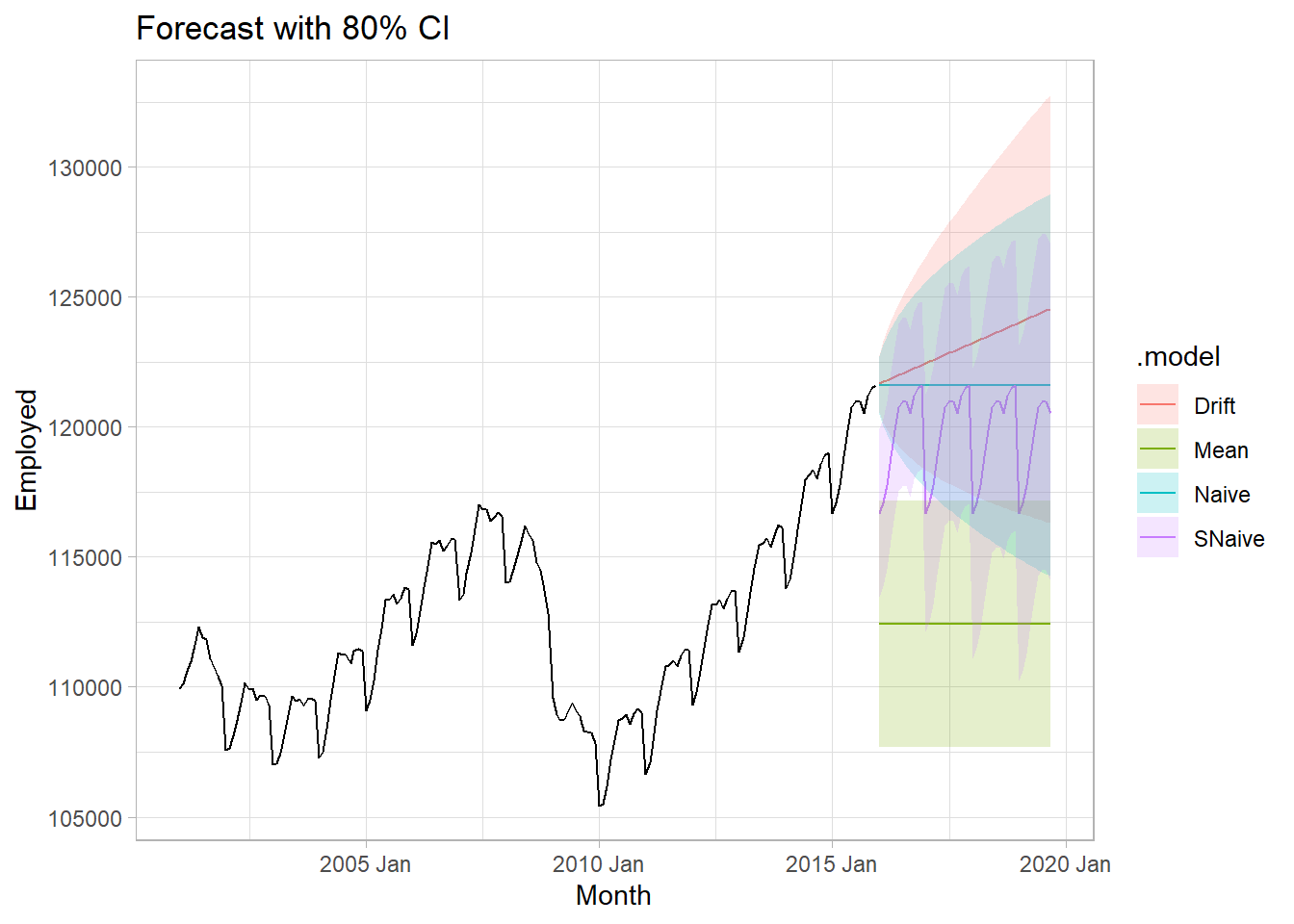
1.3 Evaluating Fit
Evaluate the model fit with residuals diagnostics.1 broom::augment() adds three columns to the model cols: .fitted, .resid, and .innov. .innov is the residual from the transformed data (if no transformation, it just equals .resid).
Innovation residuals should be independent random variables normally distributed with mean zero and constant variance (the normality and variance conditions are only required for inference and prediction intervals). Happily, feasts has just what you need.
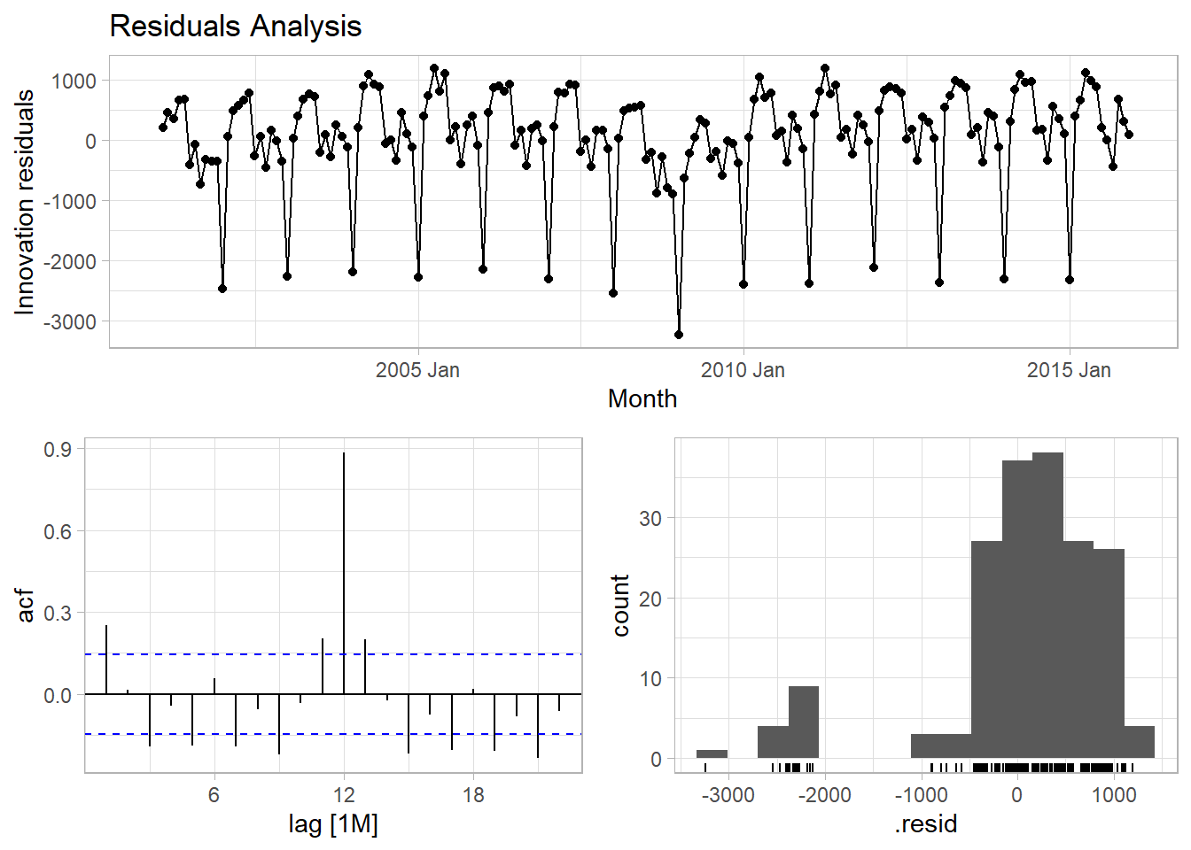
The autocorrelation plot tests the independence assumption. The histogram plot tests normality. The residuals plot tests mean zero and constant variance. You can carry out a portmanteau test on the autocorrelation assumption. Two common tests are the Box-Pierce and the Ljung-Box. These tests check the likelihood of a combination of autocorrelations at once, without testing any one correlation, kind of like an ANOVA test. The Ljung-Box test statistic is a sum of squared \(k\)-lagged autocorrelations, \(r_k^2\),
\[Q^* = T(T+2) \sum_{k=1}^l(T-k)^{-1}r_k^2.\]
The test statistic has a \(\chi^2\) distribution with \(l - K\) degrees of freedom (where \(K\) is the number of parameters in the model). Use \(l = 10\) for non-seasonal data and \(l = 2m\) for seasonal data. If your model has no explanatory variables, \(K = 0.\) Reject the no-autocorrelation (i.e., white noise) assumption if p < .05.
## # A tibble: 4 × 4
##   Title         .model lb_stat  lb_pvalue
##   <chr>         <chr>    <dbl>      <dbl>
## 1 Total Private Drift     43.3 0.00000442
## 2 Total Private Mean    1085.  0
## 3 Total Private Naive     43.3 0.00000442
## 4 Total Private SNaive  1170.  0
1.4 Model Selection
Evaluate the forecast accuracy with the test data (aka, “hold-out set”, and “out-of-sample data”). The forecast error is the difference between the observed and forecast value, \(e_{T+h} = y_{T+h} - \hat{y}_{t+h|T}.\) Forecast errors differ from model residuals in that they come from the test data set and because forecast values are usually multi-step forecasts which include prior forecast values as inputs.
The major accuracy benchmarks are:
- MAE. Mean absolute error, \(mean(|e_t|)\)
- RMSE. Root mean squared error, \(\sqrt{mean(e_t^2)}\)
- MAPE. Mean absolute percentage error, \(mean(|e_t / y_t|) \times 100\)
- MASE. Mean absolute scaled error, \(MAE/Q\) where \(Q\) is a scaling constant calculated as the average one-period change in the outcome variable (error from a one-step naive forecast).
The MAE and RMSE are on the same scale as the data, so they are only useful for comparing models fitted to the same series. MAPE is unitless, but does not work for \(y_t = 0\), and it assumes a meaningful zero (ratio data). MASE is most useful for comparing data sets of different units.
Use accuracy() to evaluate a model.
tv_fit %>%
  fabletools::forecast(new_data = tv_test) %>%
  fabletools::accuracy(data = tv_test) %>%
  select(.model, RMSE, MAE, MAPE, MASE)
## # A tibble: 4 × 5
## .model RMSE MAE MAPE MASE
## <chr> <dbl> <dbl> <dbl> <dbl>
## 1 Drift 2888. 2439. 1.93 NaN
## 2 Mean 13018. 12713. 10.1 NaN
## 3 Naive 4514. 3831. 3.02 NaN
## 4 SNaive 5961. 5435. 4.31 NaNTime series cross-validation is a better way to evaluate a model. It breaks the dataset into multiple training sets by setting a cutoff at varying points and setting the test set to a single step ahead of the horizon. Function stretch_tsibble() creates a tsibble of initial size .init and appends additional data sets of increasing size .step. Normal cross-validation repeatedly fits a model to the data set with one of the rows left out. Since model() fits a separate model per index value, creating this long tsibble effectively accomplishes the same thing. Note the fundamental difference here though: time series CV does not leave out single values from points along the time series. It leaves out all points after a particular point along the time series - each sub-data set starts at the beginning and is uninterrupted until reaching the varying end points.
us_employment_tsibble %>%
  filter(Title == "Total Private") %>%
  stretch_tsibble(.init = 3, .step = 1) %>%
  # Fit a model for each key
  model(
    Mean = MEAN(Employed),
    Naive = NAIVE(Employed),
    SNaive = SNAIVE(Employed),
    Drift = RW(Employed ~ drift())
  ) %>%
  fabletools::forecast(h = 12) %>%
  fabletools::accuracy(data = tv_test)
## # A tibble: 4 × 11
## .model Title .type ME RMSE MAE MPE MAPE MASE RMSSE ACF1
## <chr> <chr> <chr> <dbl> <dbl> <dbl> <dbl> <dbl> <dbl> <dbl> <dbl>
## 1 Drift Total Private Test 712. 1749. 1420. 0.561 1.14 0.631 0.775 0.825
## 2 Mean Total Private Test 11845. 12043. 11845. 9.43 9.43 5.27 5.33 0.822
## 3 Naive Total Private Test 1169. 2023. 1685. 0.925 1.34 0.749 0.896 0.795
## 4 SNaive Total Private Test 2267. 2274. 2267. 1.81 1.81 1.01 1.01 0.641Residuals and errors are not the same thing. The residual is the difference between the observed and fitted value in the training data set. The error is the difference between the observed and fitted value in the test data set.↩︎