2.1 Pre-processing
Chapter 1 cleaned the text. The next step is to create a document-term matrix (DTM). A DTM has one row per per document, one column per term, and frequencies in the cells. Even with stop words removed, the DTM contains mostly infrequently used terms that would not contribute to topics, so remove its sparse terms. The pre-processing steps are the same for LDA and STM with the exception of the final DTM object class.
The LDA and STM model fitting functions in this chapter use different DTM objects. topicmodels::LDA() uses class DocumentTermMatrix from the tm package. stm::stm() uses class dfm from the quanteda package. DFM stands for document feature matrix. DTM and DFM are essentially the same thing.
Keep only the decent sized reviews, ones with at least 25 words. If this is a predictive model, now is the time to create a train/test split. Consider weighting the split by the outcome variable of interest, rating in this case, to ensure proportional coverage.
set.seed(12345)

hotel_gte25 <- prepped_hotel %>% filter(prepped_wrdcnt >= 25)
nrow(hotel_gte25)
## [1] 973

# Parameter `strata` ensures proportional coverage of ratings.
hotel_split <- rsample::initial_split(hotel_gte25, prop = 3/4, strata = rating)

hotel_train <- training(hotel_split)
nrow(hotel_train)
## [1] 729

hotel_test <- testing(hotel_split)
nrow(hotel_test)
## [1] 244

token_train <- token %>% semi_join(training(hotel_split), by = join_by(review_id))

token_test <- token %>% semi_join(testing(hotel_split), by = join_by(review_id))
Most words add little value to a topic model because they appear infrequently or too frequently. The most common metric for removing sparse terms is the term frequency-inverse document frequency (TF-IDF). TF(t,d) is term t’s usage proportion in document d. IDF(t) is the log of the inverse of the term t’s proportion of documents it appears. For example, “savoy” appears in n = 109 of the N = 729 training documents. Its IDF is log(N/n) = 1.90. “savoy” appears in review #16954 in 2 of 32 (6.25%) of the terms. The TF-IDF score is the product of the two numbers. Here is that prepped review.
manage night savoy experience superb moment arrive greet experience departure staff fantastic cupcake tea coffee cocktail delicious room expect faultless comfortable breakfast wonderful experience list item breakfast world forward opportunity savoy night
Nagelkerke (2020) suggests another route. You already removed the stop words, so the over-used words are out. The TF-IDF approach was developed for long documents. Smaller documents like online reviews have little TF variation (most words are used only once or twice in a review), and the IDF ends up dominating. Instead, just filter on each word’s corpus frequency.
In the end, you need to experiment to find the right cutoff. Using TF-IDF, the elbow in the plot below is around .15. Using that threshold throws out about about 90% of the vocabulary. The corpus frequency plot has an elbow around 4 occurrences. That threshold throws out 80% of the vocabulary.
hotel_word_stats <-
  token_train %>%
  count(review_id, word, name = "doc_freq") %>%
  bind_tf_idf(word, review_id, doc_freq) %>%
  mutate(.by = word, corp_freq = sum(doc_freq)) %>%
  mutate(corp_pct = corp_freq / sum(doc_freq))

hotel_word_stats %>%
  mutate(tf_idf_bin = cut(tf_idf, breaks = 50)) %>%
  summarize(.by = tf_idf_bin, vocab = n_distinct(word)) %>%
  arrange(tf_idf_bin) %>%
  mutate(pct = vocab / sum(vocab), cumpct = cumsum(pct)) %>%
  ggplot(aes(x = tf_idf_bin)) +
  geom_col(aes(y = pct)) +
  geom_line(aes(y = cumpct, group = 1)) +
  geom_vline(xintercept = 13, linetype = 2) +
  labs(y = "vocabulary", title = "TF-IDF Method") +
  scale_y_continuous(breaks = seq(0, 1, .1), labels = percent_format(1)) +
  theme(axis.text.x = element_text(angle = 90, vjust = .5))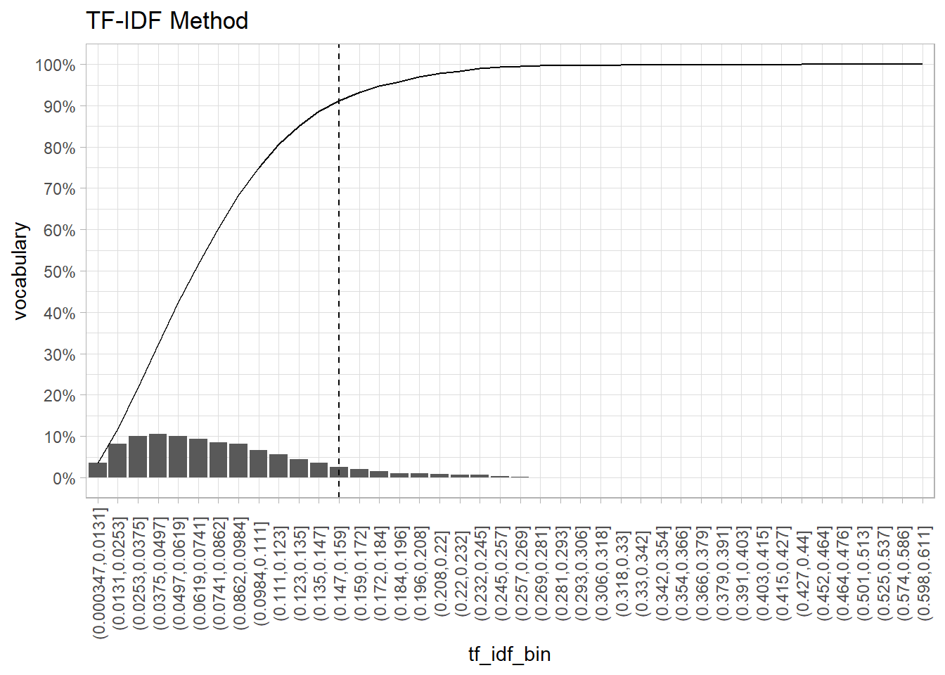
hotel_word_stats %>%
  mutate(
    corp_freq_bin = if_else(corp_freq > 19, "20+", as.character(corp_freq)),
    corp_freq_bin = factor(corp_freq_bin, levels = c(as.character(1:19), "20+"))
  ) %>%
  # mutate(corp_pct_bin = cut(corp_pct, breaks = 100)) %>%
  summarize(.by = corp_freq_bin, vocab = n_distinct(word)) %>%
  arrange(corp_freq_bin) %>%
  mutate(pct = vocab / sum(vocab), cumpct = cumsum(pct)) %>%
  ggplot(aes(x = corp_freq_bin, y = cumpct)) +
  geom_col(aes(y = pct)) +
  geom_line(aes(y = cumpct, group = 1)) +
  geom_vline(xintercept = 4, linetype = 2) +
  labs(y = "vocabulary", title = "Corpus Frequency Method") +
  scale_y_continuous(breaks = seq(0, 1, .1), labels = percent_format(1)) +
  theme(axis.text.x = element_text(angle = 90, vjust = .5))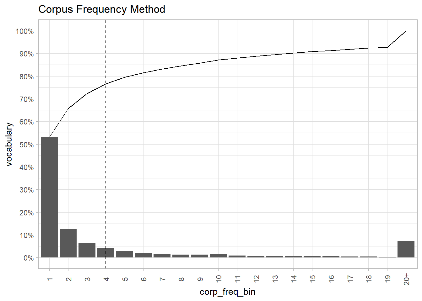
Compare the resulting DTMs. The TF-IDF method keeps half the documents and 1,500 terms. The corpus frequency method retains all documents while limiting the vocabulary to 1,200 terms. Corpus frequency does seem superior.
(dtm_tfidf <-
  hotel_word_stats %>%
  filter(tf_idf > .15) %>%
  cast_dtm(document = review_id, term = word, value = doc_freq))
## <<DocumentTermMatrix (documents: 426, terms: 1560)>>
## Non-/sparse entries: 1754/662806
## Sparsity           : 100%
## Maximal term length: 26
## Weighting          : term frequency (tf)

(dtm_corpfreq <-
  hotel_word_stats %>%
  filter(corp_freq > 5) %>%
  cast_dtm(document = review_id, term = word, value = doc_freq))
## <<DocumentTermMatrix (documents: 729, terms: 1211)>>
## Non-/sparse entries: 31208/851611
## Sparsity           : 96%
## Maximal term length: 14
## Weighting          : term frequency (tf)
The pre-processing step sure pares down the corpus. The high frequency terms comprise only 20% of the vocabulary, but are still 83% of the total word usage.
bind_rows(
  `high freq words` = hotel_word_stats %>% filter(corp_freq > 5) %>%
    summarize(distinct_words = n_distinct(word), total_words = sum(doc_freq)),
  `low freq words` = hotel_word_stats %>% filter(corp_freq <= 5) %>%
    summarize(distinct_words = n_distinct(word), total_words = sum(doc_freq)),
  .id = "partition"
) %>%
  mutate(total_pct = total_words / sum(total_words) * 100,
         distinct_pct = distinct_words / sum(distinct_words) * 100) %>%
  select(partition, distinct_words, distinct_pct, total_words, total_pct) %>%
  janitor::adorn_totals()
## partition distinct_words distinct_pct total_words total_pct
## high freq words 1211 20.41126 38093 83.15252
## low freq words 4722 79.58874 7718 16.84748
## Total 5933 100.00000 45811 100.00000