2.3 STM
STM introduces covariates which “structure” the prior distributions in the topic model Roberts et al. (2014). Topics can be correlated, each document has its own prior distribution over topics, and word use can vary by covariates. STM models incorporate two effects.
- Topical prevalence covariate effects. STM models prevalence as a function of the covariates. A survey respondent’s party affiliation may affect which topics they discuss in a question about their view on immigration. In our hotel case study, a local (UK) business traveler might care about different hotel qualities than a foreign tourist.
- Topical content covariate effects. STM models content as a function of the covariates. A survey respondent’s party affiliate may affect how they discuss topics in a question about public protests. A conservative might use words like “rioters” and “law and order” for a topic about violent demonstrations while a liberal might use words like “police brutality” and “oppression”. In the hotel example, negative reviews might focus on lapses in baseline expectations such as “sheets”, while positive reviewers focus on unexpected delights such as “origami” towels.
STM is similar to LDA in that it assumes each document is created by a generative process where topics are included according to probabilities (topical prevalence) and words are included in the topics (topical content) according to probabilities. In LDA, topic prevalence and content came from Dirichlet distributions with hyperparameters set in advance, sometimes referred to as a and b. With STM, the topic prevalence and content come from document metadata. The covariates provide a way of “structuring” the prior distributions in the topic model, injecting valuable information into the inference procedure (tingly2014?).
Fit
Fit the STM model with stm::stm(). It uses the quanteda dfm data class.1
You can cast hotel_word_stats as a DFM with tidytext::cast_dfm(), but stm() returned errors with prevalence and topic covariates. Instead, use stm::textProcessor() and stm::prepDocuments().
stm::textProcessor() produces a list object containing a vocabulary vector, a list of mini-DTM matrices for each document, and a metadata data frame. textProcessor() can remove stop words and change case, etc., but we already did that, so set those parameters to FALSE. stm::prepDocuments() removes sparse terms from the matrix.
# This produces errors in modeling phase, so don't use it.
hotel_dfm_tidy <-
  hotel_word_stats %>%
  filter(corp_freq > 5) %>%
  cast_dfm(document = review_id, term = word, value = doc_freq)

hotel_processed <-
  stm::textProcessor(
    documents = training(hotel_split) %>% pull(prepped_review),
    metadata = training(hotel_split) %>% select(rating, reviewer_loc),
    lowercase = FALSE,
    removestopwords = FALSE,
    removenumbers = FALSE,
    removepunctuation = FALSE,
    stem = FALSE
  )
## Building corpus...
## Creating Output...hotel_dfm <-
stm::prepDocuments(
hotel_processed$documents,
hotel_processed$vocab,
hotel_processed$meta,
lower.thresh = 5
)## Removing 4680 of 5814 terms (7476 of 37744 tokens) due to frequency
## Your corpus now has 729 documents, 1134 terms and 30268 tokens.What constitutes a “good” model? The topics should be cohesive in the sense that high-probability words tend to co-occur with documents. The topics should also be exclusive in the sense that the top words in topics are unlikely to be shared. To find the best model, generate a candidate set with varying tuning parameters, initialization, and pre-processing. Plot the coherence and exclusivity to identify the one with the best combination.
Take time to validate the model by trying to predict covariate values from the text.
Either specify the number of topics (K) to identify, or let stm() choose an optimal number by setting K = 0. The resulting probability distribution of topic words (beta matrix) will be a K x 5,814 matrix. The probability distribution of topics (gamma matrix, theta in the stm package) will be a 729 x K matrix. I expect topics to correlate with the review rating, so rating is a prevalence covariate, and I expect word usage to correlate with the reviewer location, so reviewer_loc is a topical content covariate.
# This model fit operation took 15 minutes to run. Run once and save to disk.
set.seed(1234)

stm_fits <-
  tibble(K = seq(from = 2, to = 10, by = 2)) %>%
  mutate(fit = map(
    K,
    ~stm::stm(
        documents = hotel_dfm$documents,
        vocab = hotel_dfm$vocab,
        K = .,
        prevalence = ~ rating,
        content = ~ reviewer_loc,
        data = hotel_dfm$meta,
        verbose = FALSE
      )
  ))

stm_fit <- stm::stm(
  documents = hotel_dfm$documents,
  vocab = hotel_dfm$vocab,
  K = 4,
  prevalence = ~ rating,
  content = ~ reviewer_loc,
  data = hotel_dfm$meta,
  verbose = FALSE
)

saveRDS(stm_fit, file = "input/stm_fit.RDS")## Length Class Mode
## documents 729 -none- list
## vocab 1134 -none- character
## meta 2 data.frame list
## words.removed 4680 -none- character
## docs.removed 0 -none- NULL
## tokens.removed 1 -none- numeric
## wordcounts 5814 -none- numericWhereas LDA models are optimized using the perplexity statistic, STM offers several options. The most useful are the held-out likelihood and coherence.
stm_heldout <- stm::make.heldout(hotel_dfm$documents, vocab = hotel_dfm$vocab)

stm::semanticCoherence(stm_fit, documents = hotel_dfm$documents)

stm_fits %>%
  mutate(
    semantic_coherence = map(fit, ~semanticCoherence(.x, documents = hotel_dfm$documents))
  ) %>%
  select(K, semantic_coherence) %>%
  unnest(semantic_coherence) %>%
  summarize(.by = K, semantic_coherence = mean(semantic_coherence)) %>%
  ggplot(aes(x = K, y = semantic_coherence)) +
    geom_line()

stm_fit2 <- stm::stm(
  stm_heldout$documents,
  stm_heldout$vocab,
  K = 4,
  prevalence = ~ rating,
  content = ~ reviewer_loc,
  data = hotel_dfm$meta,
  init.type = "Spectral",
  verbose = FALSE
)

# stm_fit2 %>% stm::exclusivity()
# stm_fit2 %>% stm::semanticCoherence(documents = stm_heldout$documents)
Interpret
The fit summary has three sections showing the tops words. The first section shows the prevalence model; the second shows the topical content model; and the third shows their interaction.
## A topic model with 4 topics, 729 documents and a 1134 word dictionary.## Topic Words:
## Topic 1: ham, bean, sausage, owner, chair, cereal, liverpool
## Topic 2: covent, trafalgar, piccadilly, victoria, square, oxford, rembrandt
## Topic 3: incredible, amaze, rumpus, knowledgeable, kaspers, overlook, cocktail
## Topic 4: seafood, savoy, medium, remove, simply, foyer, grill
##
## Covariate Words:
## Group Other: daily, market, vacation, internet, awesome, closet, hope
## Group United Kingdom: cook, ooze, downside, party, finish, weekend, wife's
## Group United States: handle, garden, london's, sightsee, plush, server, prompt
##
## Topic-Covariate Interactions:
## Topic 1, Group Other: rees, wifi, ensuite, ridgemount, window, gower, chris
## Topic 1, Group United Kingdom: gown, ben, escape, stain, secret, smell, corridor
## Topic 1, Group United States: warn, soap, driver, screen, pauls, overlook, flat
##
## Topic 2, Group Other: hop, ben, min, transportation, directly, heathrow, line
## Topic 2, Group United Kingdom: rate, contemporary, furnish, spotlessly, honest, dcor, central
## Topic 2, Group United States: market, paris, strong, rees, knowledgeable, unique, june
##
## Topic 3, Group Other: spa, pricey, sandwich, dorchester, cake, beautiful, champagne
## Topic 3, Group United Kingdom: brilliant, 15th, sister, deco, 14th, wed, minibar
## Topic 3, Group United States: freshly, massive, rate, outlet, appoint, traveller, butler
##
## Topic 4, Group Other: junior, server, call, follow, difference, fix, happen
## Topic 4, Group United Kingdom: sandwich, frankly, ambience, plush, surrounding, scone, excite
## Topic 4, Group United States: beautifully, deco, plan, venue, beaufort, seafood, grill
## If this was just a regular topic model, or a prevalence or content model, we’d see top words by 4 metrics: highest probability, FREX, lift, and score.
- Highest probability weights words by their overall frequency.
- FREX weights words by their overall frequency and how exclusive they are to the topic.
- Lift weights words by dividing by their frequency in other topics, therefore giving higher weight to words that appear less frequently in other topics.
- Score divides the log frequency of the word in the topic by the log frequency of the word in other topics.
Let’s fit a new model just to show that.
set.seed(1234)

stm_fit_simple <- stm::stm(
  hotel_dfm$documents,
  hotel_dfm$vocab,
  K = 4,
  # prevalence = ~ rating,
  # content = ~ reviewer_loc,
  data = hotel_dfm$meta,
  init.type = "Spectral",
  verbose = FALSE
)

saveRDS(stm_fit_simple, file = "input/stm_fit_simple.RDS")## Topic 1 Top Words:
## Highest Prob: stay, london, staff, service, excellent, restaurant, location
## FREX: spa, corinthia, concierge, luxury, mondrian, love, pool
## Lift: personal, oriental, mandarin, notch, corinthia, pleasure, property
## Score: personal, london, service, stay, spa, corinthia, location
## Topic 2 Top Words:
## Highest Prob: breakfast, walk, room, stay, location, clean, london
## FREX: tube, station, museum, hyde, street, bus, walk
## Lift: hyde, paddington, albert, ridgemount, bus, kensington, rhodes
## Score: hyde, tube, station, museum, bus, walk, clean
## Topic 3 Top Words:
## Highest Prob: savoy, bar, tea, lovely, staff, special, birthday
## FREX: afternoon, birthday, savoy, cocktail, cake, american, treat
## Lift: scone, pianist, cake, piano, beaufort, afternoon, sandwich
## Score: scone, savoy, afternoon, birthday, tea, cake, cocktail
## Topic 4 Top Words:
## Highest Prob: room, night, check, stay, bed, book, bathroom
## FREX: check, charge, bath, call, floor, pay, issue
## Lift: rumpus, robe, mirror, wake, smell, curtain, corridor
## Score: rumpus, room, check, shower, bed, bathroom, floorIt is interesting that the top terms for UK did not include “restaurant” or “location”. The top terms for the US did not include “excellent” or “amaze”, but did include “love”.
stm_tidy <- tidy(stm_fit)

stm_top_tokens <-
  stm_tidy %>%
  mutate(topic = factor(paste("Topic", topic))) %>%
  group_by(topic, y.level) %>%
  slice_max(order_by = beta, n = 10) %>%
  ungroup()

stm_top_tokens %>%
  filter(topic == "Topic 1") %>%
  ggplot(aes(x = beta, y = reorder_within(term, by = beta, within = topic))) +
  geom_col() +
  scale_y_reordered() +
  facet_wrap(facets = vars(y.level), scales = "free_x", ncol = 3) +
  labs(y = NULL, title = "STM Top 10 Terms for Topic 1")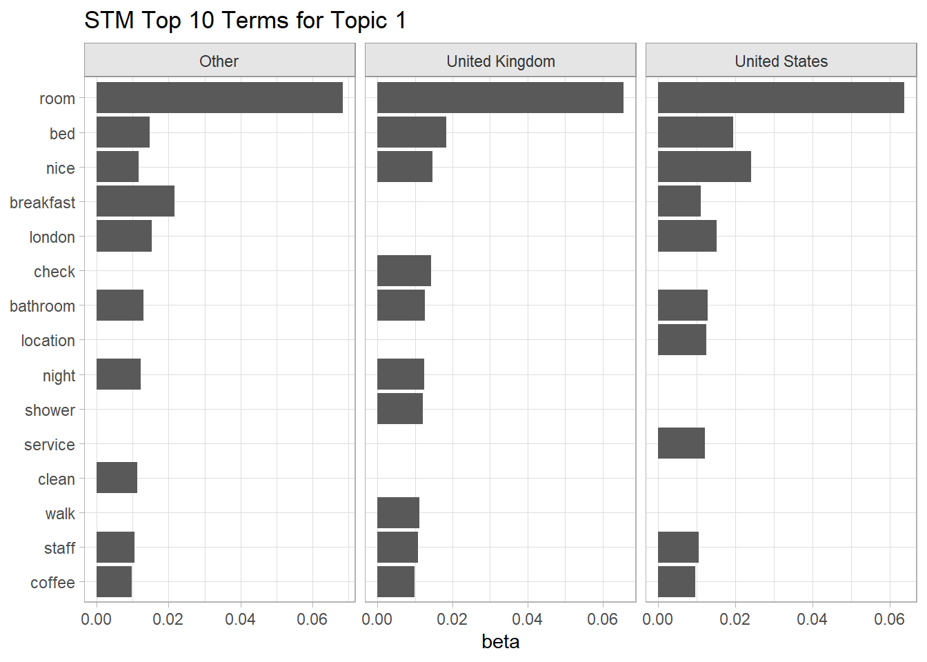
As we did with the LDA model, we can assign topic labels with Open AI.
stm_topics <-
  stm_top_tokens %>%
  nest(data = term, .by = topic) %>%
  mutate(
    token_str = map(data, ~paste(.$term, collapse = ", ")),
    topic_lbl = map_chr(token_str, get_topic_from_openai),
    topic_lbl = str_remove_all(topic_lbl, '\\"'),
    topic_lbl = snakecase::to_any_case(topic_lbl, "title")
  ) %>%
  select(-data)

# Save to file system to avoid regenerating.
saveRDS(stm_topics, file = "input/stm_topics.RDS")## # A tibble: 4 × 3
## topic token_str topic_lbl
## <fct> <list> <chr>
## 1 Topic 1 <chr [1]> Luxury Stay in London
## 2 Topic 2 <chr [1]> Comfortable Stay Near London
## 3 Topic 3 <chr [1]> Afternoon Tea at the Savoy
## 4 Topic 4 <chr [1]> Hotel StayAnother way to evaluate the model is to print reviews that are most representative of the topic. Topic 1
stm::findThoughts(
  stm_fit,
  n = 3,
  texts = hotel_dfm$meta$review,
  topics = 1,
  meta = hotel_dfm$meta
)
## Warning in stm::findThoughts(stm_fit, n = 3, texts = hotel_dfm$meta$review, :
## texts are of type 'factor.' Converting to character vectors. Use
## 'as.character' to avoid this warning in the future.##
## Topic 1:
## United Kingdom
## Other
## United KingdomReferences
I used STM for my Battle of the Bands project.↩︎