Suppose you run an experiment measuring the effect of two types of secondary tasks on the time it takes a person to complete a primary task. This is normally a good candidate for a linear regression, but there is a twist: the participants each generate many data points, and they naturally vary in their multitasking skills. This twist violates the independent observations assumption. What to do? The solution is linear mixed effects models (LMMs).1
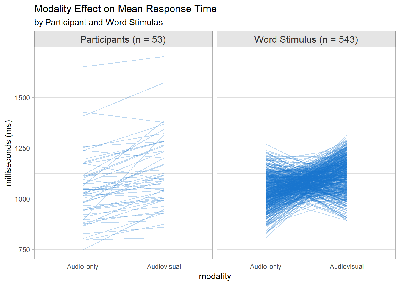
The datasets are from a study about multi-tasking. In rt_dat, the researchers measured participant (PID) response time (RT) on a primary task while completing a secondary task of repeating words presented in one of two modalities (modality): audio-only and audiovisual. The researchers hypothesized that the higher cognitive load associated with audiovisual stimulation would increase RT. Each participant repeated the experiment with various words (stimulus, stim). In acc_dat, the dependent variable is response accuracy (acc\(\in [0,1]\)) rather than response time.
There were 53 participants and 543 words. The summary table suggests audiovisual modality does indeed retard response times over audio-only.
PID and stim are important covariates because people differ in their ability to multitask, and words vary in difficulty.
Show the code
bind_rows(Participants =summarize(rt_dat, .by =c(modality, PID), M =mean(RT)),Stimulus =summarize(rt_dat, .by =c(modality, stim), M =mean(RT)),.id ="Factor") |>mutate(Factor =case_when( Factor =="Participants"~glue("Participants (n = {n_PID})"), Factor =="Stimulus"~glue("Word Stimulus (n = {n_stim})") ),grp =coalesce(PID, stim) ) %>%ggplot(aes(x = modality)) +geom_line(aes(y = M, group = grp), alpha = .3, color ="dodgerblue3") +facet_wrap(facets =vars(Factor)) +labs(title ="Modality Effect on Mean Response Time",subtitle ="by Participant and Word Stimulas",y ="milliseconds (ms)" )
3.1 LMM Model
Mixed-effects models are called “mixed” because they simultaneously model fixed and random effects. Fixed effects are population-level effects that should persist across experiments. Fixed effects are the traditional predictors in a regression model. modality is a fixed effect. Random effects are level effects that account for variability at different levels of the data hierarchy. PID and stim are random effects because they are randomly sampled and you expect variability within the populations.
LMM represents the \(i\)-th observation for the \(j\)-th random-effects group as
Where \(\beta_0\) and \(\beta_1\) are the fixed effect intercept and slope, and \(u_j\) is the random effect for the \(j\)-th group. The \(u_j\) terms are the group deviations from the population mean and are assumed to be normally distributed with mean 0 and variance \(\sigma_u^2\). The residual term is also assumed to be normally distributed with mean 0 and variance \(\sigma_\epsilon^2\)
In our study, \(\beta_0\) and \(\beta_1\) are the fixed effects of modality; \(u_j\) is the \(j\) = 53 PID levels; and the model includes an additional term, \(\eta_k\), for the \(k\) = 543 stim levels.
Fit an LMM with the lmer package. The pipes (|) in the formula indicate the value to the left varies by the variable to the right. 1 is the intercept (no interactions). You can model the random effects two ways:
(1|PID) + (1|stim): level effects by participant and stimulus.
Linear mixed model fit by REML ['lmerMod']
Formula: RT ~ 1 + modality + (1 | PID) + (1 | stim)
   Data: data

REML criterion at convergence: 302861.5

Scaled residuals:
    Min      1Q  Median      3Q     Max
-3.3572 -0.6949 -0.0205  0.5814  4.9120

Random effects:
 Groups   Name        Variance Std.Dev.
 stim     (Intercept)   360.2   18.98
 PID      (Intercept) 28065.7  167.53
 Residual             67215.3  259.26
Number of obs: 21679, groups:  stim, 543; PID, 53

Fixed effects:
                    Estimate Std. Error t value
(Intercept)         1044.449     23.164   45.09
modalityAudiovisual   82.525      3.529   23.38

Correlation of Fixed Effects:
            (Intr)
modltyAdvsl -0.078
Let’s walk through these sections.
Tip
Use broom.mixed::tidy() to pull the coefficient estimates.
(tidy_fit <- broom.mixed::tidy(rt_fit_1))
# A tibble: 5 × 6
  effect   group    term                estimate std.error statistic
  <chr>    <chr>    <chr>                  <dbl>     <dbl>     <dbl>
1 fixed    <NA>     (Intercept)           1044.      23.2       45.1
2 fixed    <NA>     modalityAudiovisual     82.5      3.53      23.4
3 ran_pars stim     sd__(Intercept)         19.0     NA         NA
4 ran_pars PID      sd__(Intercept)        168.      NA         NA
5 ran_pars Residual sd__Observation        259.      NA         NA
The Random effects show the variability in RT due to stim and PID. The variability among participants (PID sd = 168 ms) is much greater than the variability among words (stim sd = 19 ms).
The Fixed effects show audio-visual modality slows RT by 82.5 ms over audio-only.
The Correlation of Fixed Effects shows a weak negative correlation between the intercept and the audio-visual modality effect (modltyAdvsl = -0.078 ms). This means when RT times were high, audiovisual effect was somewhat diminished.
To add interactions between the fixed effect variable(s) and the random effects variable(s), change the random intercept (1) to the fixed effect variable. Then both the intercept and the slope can vary.
Linear mixed model fit by REML ['lmerMod']
Formula: RT ~ 1 + modality + (1 + modality | PID) + (1 + modality | stim)
   Data: data

REML criterion at convergence: 302385.7

Scaled residuals:
    Min      1Q  Median      3Q     Max
-3.3646 -0.6964 -0.0141  0.5886  5.0003

Random effects:
 Groups   Name                Variance Std.Dev. Corr
 stim     (Intercept)           304.0   17.44
          modalityAudiovisual   216.9   14.73   0.16
 PID      (Intercept)         28559.0  168.99
          modalityAudiovisual  7709.0   87.80   -0.17
 Residual                     65258.8  255.46
Number of obs: 21679, groups:  stim, 543; PID, 53

Fixed effects:
                    Estimate Std. Error t value
(Intercept)          1044.14      23.36  44.700
modalityAudiovisual    83.18      12.57   6.615

Correlation of Fixed Effects:
            (Intr)
modltyAdvsl -0.178
This formulation includes random slopes for modality within PID and stim, meaning you’re accounting for differences in how each participant and stimulus responds to modality. Response times varied around 1,044 ms by sd = 17 ms for stim and sd = 169 ms for PID. The modality effect on response times varied around 83 ms by sd = 15 ms for stim and sd = 88 ms for PID. That last statistic means a participant whose slope is 1 sd below the mean would have a slope near zero - a modality effect of zero.
The added correlations in the Random effects section show how the intercept and slopes for modality vary together within each group. The 0.16 correlation between the stimuli and fixed-effect intercepts indicates that stimuli with longer response times in the audio modality tended to have more positive slopes (stronger positive audiovisual effect). The -0.17 correlation between the participant and fixed-effect intercepts indicates that participants with longer response times in the audio modality tended to have a less positive slope (weaker positive, or possibly even a negative, audiovisual effect).
The audio-visual modality slows RT by 83 ms over audio-only - same as in the first model. The REML criterion fell, so adding the random slopes for modality improved the fit.
3.3 Assumptions
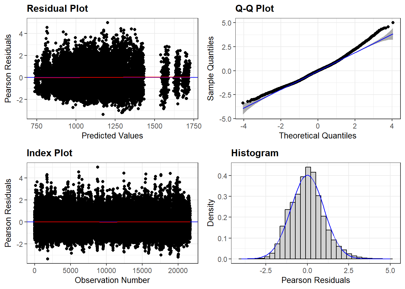
The linear regression model assumptions still apply: the relationship between the predictors and the response is linear and the residuals are independent random variables normally distributed with mean zero and constant variance. Additionally, the the random effects intercepts and slopes are assumed to follow a normal distribution. Use residual plots to assess linearity, homoscedasticity, and independence. Use Q-Q plots to check the normality of residuals and random effects. Variance inflation factors (VIFs) can help detect multicollinearity among predictors.
To determine whether the modality fixed effect actually affected response times, compare the model to a nested model without modality using a likelihood-ratio test. Likelihood ratio tests calculating the likelihoods for the models using maximum likelihood estimation then compares those likelihoods. A significant test results indicates the full model fit the data better. Perform a likelihood ratio test anova().
# A tibble: 2 × 9
  term            npar    AIC    BIC  logLik minus2logL statistic    df  p.value
  <chr>          <dbl>  <dbl>  <dbl>   <dbl>      <dbl>     <dbl> <dbl>    <dbl>
1 extract_fit_e…     8 3.02e5 3.03e5 -1.51e5    302433.      NA      NA NA
2 extract_fit_e…     9 3.02e5 3.02e5 -1.51e5    302401.      32.4     1  1.26e-8
, but there is a better way. afex::mixed(method = "LRT") performs the test for all fixed effects variables in the model. In this case study we have only one.
The likelihood-ratio test indicated that the model including modality provided a better fit for the data than a model without it, \(\chi^2\)(1) = 32.4, p < .001.
A likelihood-ratio test indicated that the model including modality provided a better fit for the data than a model without it, \(\chi^2\)(1) = 32.4, p < .001. Examination of the summary output for the full model indicated that response times were on average an estimated 83.2 ms slower in the audiovisual relative to the audio-only condition (\(\hat{\beta}\) = 83.2, SE = 12.6, t = 83.2, SE = 6.6).
gtsummary::tbl_regression(rt_fit_2)
Characteristic
Beta
95% CI
modality
Audio-only
—
—
Audiovisual
83
59, 108
Abbreviation: CI = Confidence Interval
3.6 Logistic Regression
This section fits a logistic LMM to the acc_dat dataset.
Or maybe pre-summarize the data by calculating the mean response time across all words by PID and modality, then run the regression controlling for just PID.
Show the code
x <-summarize(rt_dat, .by =c(modality, PID), MRT =mean(RT))linear_reg() |>fit(MRT ~ modality + PID, data = x) |>tidy() |>filter(!str_detect(term, "^PID"))
Brown, Violet A. 2021. “An Introduction to Linear Mixed-Effects Modeling in r.”Advances in Methods and Practices in Psychological Science 4 (1): 2515245920960351. https://doi.org/10.1177/2515245920960351.
Another option is repeated measures ANOVA. However, repeated measures ANOVA can model either participant or item variability, but not both simultaneously. Also, ANOVA requires continuous outcomes and ccategorical predictors.↩︎
The article is a good tutorial and worth reading.↩︎
Source Code
# Mixed Effects Models```{r setup}#| include: falselibrary(tidyverse)library(glue)library(tidymodels)library(gtsummary)tidymodels_prefer()library(multilevelmod)library(ggResidpanel)theme_set( theme_light() + theme( plot.caption = element_text(hjust = 0), strip.background = element_rect(fill = "gray90", color = "gray60"), strip.text = element_text(color = "gray20", size = 12) ))```Suppose you run an experiment measuring the effect of two types of secondary tasks on the time it takes a person to complete a primary task. This is normally a good candidate for a linear regression, but there is a twist: the participants each generate many data points, and they naturally vary in their multitasking skills. This twist violates the _independent observations_ assumption. What to do? The solution is *linear mixed effects models* (LMMs).[^lmer-1][^lmer-1]: Another option is repeated measures ANOVA. However, repeated measures ANOVA can model either participant or item variability, but not both simultaneously. Also, ANOVA requires continuous outcomes and ccategorical predictors.We'll work with a datasets included in the [supplemental materials](https://osf.io/v6qag/) of *An Introduction to Linear Mixed-Effects Modeling* [@Brown2021].[^lmer-2][^lmer-2]: The article is a good tutorial and worth reading.```{r}#| code-fold: false#| echo: truert_dat <- readr::read_csv("./input/mixed-effects-rt.csv", col_types ="cdcc") |>mutate(modality =factor(modality, levels =c("Audio-only", "Audiovisual")))acc_dat <- readr::read_csv("./input/mixed-effects-acc.csv", col_types ="cdcc") |>mutate(modality =factor(modality, levels =c("Audio-only", "Audiovisual")),acc =factor(acc) )glimpse(rt_dat)glimpse(acc_dat)```The datasets are from a study about multi-tasking. In `rt_dat`, the researchers measured participant (`PID`) response time (`RT`) on a primary task while completing a secondary task of repeating words presented in one of two modalities (`modality`): audio-only and audiovisual. The researchers hypothesized that the higher cognitive load associated with audiovisual stimulation would increase `RT`. Each participant repeated the experiment with various words (stimulus, `stim`). In `acc_dat`, the dependent variable is response accuracy (`acc` $\in [0,1]$) rather than response time.```{r}#| include: falsen_PID <-n_distinct(rt_dat$PID)n_stim <-n_distinct(rt_dat$stim)```There were `r n_PID` participants and `r n_stim` words in `rt_dat`. The summary tables suggests the audiovisual modality does indeed retard response times over audio-only, but increased accuracy.```{r}#| code-fold: true#| message: falsegtsummary::tbl_summary( rt_dat,by = modality,include =-c(PID, stim),statistic =list(gtsummary::all_continuous() ~"{mean}, {sd}")) |> gtsummary::as_gt() |> gt::tab_header(title ="rt_dat")```<br>```{r}#| code-fold: true#| message: falsegtsummary::tbl_summary( acc_dat,by = modality,include =-c(PID, stim)) |> gtsummary::as_gt() |> gt::tab_header(title ="acc_dat")```<br>`PID` and `stim` are important covariates because people differ in their ability to multitask, and words vary in difficulty.```{r}#| code-fold: truebind_rows(Participants =summarize(rt_dat, .by =c(modality, PID), M =mean(RT)),Stimulus =summarize(rt_dat, .by =c(modality, stim), M =mean(RT)),.id ="Factor") |>mutate(Factor =case_when( Factor =="Participants"~glue("Participants (n = {n_PID})"), Factor =="Stimulus"~glue("Word Stimulus (n = {n_stim})") ),grp =coalesce(PID, stim) ) %>%ggplot(aes(x = modality)) +geom_line(aes(y = M, group = grp), alpha = .3, color ="dodgerblue3") +facet_wrap(facets =vars(Factor)) +labs(title ="Modality Effect on Mean Response Time",subtitle ="by Participant and Word Stimulas",y ="milliseconds (ms)" )```## LMM ModelMixed-effects models are called “mixed” because they simultaneously model fixed and random effects. Fixed effects are population-level effects that should persist across experiments. Fixed effects are the traditional predictors in a regression model. `modality` is a fixed effect. Random effects are level effects that account for variability at different levels of the data hierarchy. `PID` and `stim` are random effects because they are randomly sampled and you expect variability within the populations.LMM represents the $i$-th observation for the $j$-th random-effects group as$$y_{ij} = \beta_0 + \beta_1x_{ij} + u_j + \epsilon_{ij}$$ {#eq-lmm-model}Where $\beta_0$ and $\beta_1$ are the fixed effect intercept and slope, and $u_j$ is the random effect for the $j$-th group. The $u_j$ terms are the group deviations from the population mean and are assumed to be normally distributed with mean 0 and variance $\sigma_u^2$. The residual term is also assumed to be normally distributed with mean 0 and variance $\sigma_\epsilon^2$In our study, $\beta_0$ and $\beta_1$ are the fixed effects of `modality`; $u_j$ is the $j$ = `r n_PID``PID` levels; and the model includes an additional term, $\eta_k$, for the $k$ = `r n_stim``stim` levels.$$y_{ij} = \beta_0 + \beta_1x_{ij} + u_j + \eta_k + \epsilon_{ijk}$$## The _lmer_ EngineFit an LMM with the _lmer_ package. The pipes (\|) in the formula indicate the value to the left varies by the variable to the right. 1 is the intercept (no interactions). You can model the random effects two ways:- `(1|PID) + (1|stim)`: level effects by participant and stimulus.- `(1 + modality|PID) + (1 + modality|stim)`: level effects plus interaction effects.Start with the level effect model.```{r fit-1}#| code-fold: falsert_fit_1 <- linear_reg() |> set_engine("lmer") |> fit( RT ~ 1 + modality + (1|PID) + (1|stim), data = rt_dat )extract_fit_engine(rt_fit_1) |> summary()```Let's walk through these sections. ::: {.callout-tip}Use `broom.mixed::tidy()` to pull the coefficient estimates.```{r}#| code-fold: false(tidy_fit <- broom.mixed::tidy(rt_fit_1))```:::- The *Random effects* show the variability in `RT` due to `stim` and `PID`. The variability among participants (`PID` sd = `r tidy_fit |> filter(group == "PID", term == "sd__(Intercept)") |> pull(estimate) |> comma()` ms) is much greater than the variability among words (`stim` sd = `r tidy_fit |> filter(group == "stim", term == "sd__(Intercept)") |> pull(estimate) |> comma()` ms).- The *Fixed effects* show audio-visual modality slows `RT` by `r tidy_fit |> filter(effect == "fixed", term == "modalityAudiovisual") |> pull(estimate) |> comma(.1)` ms over audio-only.- The *Correlation of Fixed Effects* shows a weak negative correlation between the intercept and the audio-visual modality effect (`modltyAdvsl` = `r extract_fit_engine(rt_fit_1) |> summary() |> pluck("vcov", "factors", "correlation") |> pluck("x", 3) |> comma(.001)` ms). This means when `RT` times were high, audiovisual effect was somewhat diminished.To add interactions between the fixed effect variable(s) and the random effects variable(s), change the random intercept (1) to the fixed effect variable. Then both the intercept and the slope can vary.```{r fit-2}#| code-fold: falsert_fit_2 <- linear_reg() |> set_engine("lmer") |> fit( RT ~ 1 + modality + (1 + modality|PID) + (1 + modality|stim), data = rt_dat )summary(extract_fit_engine(rt_fit_2))```This formulation includes random slopes for `modality` within `PID` and `stim`, meaning you’re accounting for differences in how each participant and stimulus responds to modality. Response times varied around `r broom.mixed::tidy(rt_fit_2) %>% filter(term == "(Intercept)") %>% pull(estimate) %>% comma(1)` ms by sd = `r broom.mixed::tidy(rt_fit_2) %>% filter(term == "sd__(Intercept)", group == "stim") %>% pull(estimate) %>% comma(1)` ms for `stim` and sd = `r broom.mixed::tidy(rt_fit_2) %>% filter(term == "sd__(Intercept)", group == "PID") %>% pull(estimate) %>% comma(1)` ms for `PID`. The modality effect on response times varied around `r broom.mixed::tidy(rt_fit_2) %>% filter(term == "modalityAudiovisual") %>% pull(estimate) %>% comma(1)` ms by sd = `r broom.mixed::tidy(rt_fit_2) %>% filter(term == "sd__modalityAudiovisual", group == "stim") %>% pull(estimate) %>% comma(1)` ms for `stim` and sd = `r broom.mixed::tidy(rt_fit_2) %>% filter(term == "sd__modalityAudiovisual", group == "PID") %>% pull(estimate) %>% comma(1)` ms for PID. That last statistic means a participant whose slope is 1 sd below the mean would have a slope near zero - a modality effect of zero.The added correlations in the *Random effects* section show how the intercept and slopes for `modality` vary together within each group. The `r broom.mixed::tidy(rt_fit_2) %>% filter(term == "cor__(Intercept).modalityAudiovisual", group == "stim") %>% pull(estimate) %>% comma(.01)` correlation between the stimuli and fixed-effect intercepts indicates that stimuli with longer response times in the audio modality tended to have more positive slopes (stronger positive audiovisual effect). The `r broom.mixed::tidy(rt_fit_2) %>% filter(term == "cor__(Intercept).modalityAudiovisual", group == "PID") %>% pull(estimate) %>% comma(.01)` correlation between the participant and fixed-effect intercepts indicates that participants with longer response times in the audio modality tended to have a less positive slope (weaker positive, or possibly even a negative, audiovisual effect).The audio-visual modality slows `RT` by `r broom.mixed::tidy(rt_fit_2) |> filter(effect == "fixed", term == "modalityAudiovisual") |> pull(estimate) |> comma()` ms over audio-only - same as in the first model. The REML criterion fell, so adding the random slopes for modality improved the fit.## AssumptionsThe linear regression model assumptions still apply: the relationship between the predictors and the response is linear and the residuals are independent random variables normally distributed with mean zero and constant variance. Additionally, the the random effects intercepts and slopes are assumed to follow a normal distribution. Use residual plots to assess linearity, homoscedasticity, and independence. Use Q-Q plots to check the normality of residuals and random effects. Variance inflation factors (VIFs) can help detect multicollinearity among predictors.```{r}#| code-fold: false#| message: falseresid_panel(extract_fit_engine(rt_fit_2), smoother =TRUE, qqbands =TRUE)```## EvaluationTo determine whether `modality` affects response times, compare the model to a nested model without `modality` using a likelihood-ratio test (LRT). LRT calculates the model likelihoods using maximum likelihood estimation then compares those likelihoods. A significant test result indicates the full model fits the data better.::: {.callout-note}### Why not rely on the Wald (coefficient t-) test?Degrees-of-freedom are tricky for mixed models and Wald *p*-values use approximations that can be unrliable in complex random structures. :::```{r rt-lrt}# reduced model exlcludes the `modality` predictor.rt_reduced <- linear_reg() |> set_engine("lmer") |> fit( RT ~ 1 + (1 + modality|PID) + (1 + modality|stim), data = rt_dat )rt_lrt <- anova( extract_fit_engine(rt_fit_2), extract_fit_engine(rt_reduced))tidy(rt_lrt)```The likelihood-ratio test indicated that the model including modality provided a better fit for the data than a model without it, $\chi^2$(1) = `r comma(rt_lrt$Chisq[2], .1)`, *p* \< .001.## Reporting```{r}#| code-fold: falseav_terms <- broom.mixed::tidy(rt_fit_2) |>filter(term =="modalityAudiovisual")```> A likelihood-ratio test indicated that the model including modality provided a better fit for the data than a model without it, $\chi^2$(1) = `r comma(rt_lrt$Chisq[2], .1)`, *p* \< .001. Examination of the summary output for the full model indicated that response times were on average an estimated `r comma(av_terms[1, ]$estimate, .1)` ms slower in the audiovisual relative to the audio-only condition ($\hat{\beta}$ = `r comma(av_terms[1, ]$estimate, .1)`, *SE* = `r comma(av_terms[1, ]$std.error, .1)`, *t* = `r comma(av_terms[1, ]$estimate, .1)`, *SE* = `r comma(av_terms[1, ]$statistic, .1)`).```{r message=FALSE}#| code-fold: falsegtsummary::tbl_regression(rt_fit_2)```## Logistic RegressionThis section fits a logistic LMM to the `acc_dat` dataset.```{r acc-fit}acc_fit <- logistic_reg() |> set_engine("glmer") |> set_mode("classification") |> fit( acc ~ 1 + modality + (1 + 1|PID) + (1 + 1|stim), data = acc_dat, family = "binomial" )```Fit a reduced model lacking the `modality` fixed effect to use in a likelihood ratio test.```{r acc-lrt}acc_reduced_fit <- logistic_reg() |> set_engine("glmer") |> set_mode("classification") |> fit( acc ~ 1 + (1 + 1|PID) + (1 + 1|stim), data = acc_dat, family = "binomial" )lrt_acc <- anova( extract_fit_engine(acc_fit), extract_fit_engine(acc_reduced_fit))tidy(lrt_acc)```