The design and analysis of a survey depends on its purpose. Exploratory surveys investigate topics with no particular expectation. They are usually qualitative and often ask open-ended questions which are analyzed for content (word/phrase frequency counts) and themes. Descriptive surveys measure the association between the survey topic(s) and the respondent attributes. They typically ask Likert scale questions. Explanatory surveys explain and quantify hypothesized relationships with inferential statistics.
In a survey project, exploratory factor analysis (EFA), item reduction, and confirmatory factor analysis (CFA) play critical roles in refining and validating the questionnaire. Here’s how they fit into the major phases of a survey project:
2.0.1 1. Survey Design and Item Development
Item Generation: During the initial design phase, you generate items (questions) based on the concepts you wish to measure. This involves creating questions that capture each domain or construct of interest.
Preliminary Item Pool: You often start with a larger pool of items than you plan to use in the final survey. The aim is to cover all relevant aspects of the constructs comprehensively, knowing that some items will be refined or removed later.
2.0.2 2. Pilot Testing and Exploratory Factor Analysis (EFA)
Pilot Survey Administration: After developing the preliminary item pool, a pilot survey is administered to a small group from the target population.
Exploratory Factor Analysis (EFA): EFA is conducted to explore the underlying structure of the data without imposing any predefined structure. This helps identify latent factors (or constructs) that the items represent and assess if the items group together as expected.
Purpose: EFA provides insights into whether items align with the hypothesized constructs or if adjustments are needed.
Outcome: The result of EFA often leads to item reduction, where redundant or low-loading items (items that don’t contribute well to the factors) are removed to create a cleaner, more interpretable structure.
2.0.3 3. Item Reduction and Refinement
Item Reduction: Based on the results from EFA, items that don’t load well on any factor or that cause cross-loading issues (loading on multiple factors) are removed. This results in a streamlined set of items that reliably measure the intended constructs.
Revised Survey Development: A revised version of the survey is developed with the refined item pool, improving clarity, reducing redundancy, and ensuring that each item is relevant to a single construct.
2.0.4 4. Field Testing and Confirmatory Factor Analysis (CFA)
Larger Sample Administration: The refined survey is then administered to a larger, more representative sample to test its reliability and validity.
Confirmatory Factor Analysis (CFA): CFA is conducted to validate the factor structure identified in the EFA phase. CFA requires specifying the number of factors and their relationships based on prior knowledge or the EFA results.
Purpose: CFA tests how well the items fit the hypothesized structure and whether the constructs align with theoretical expectations. Good model fit in CFA indicates that the items reliably measure each intended factor.
2.0.5 5. Final Survey Administration and Data Collection
With a validated survey, you can proceed to full-scale data collection, confident that the items are reliable and valid measures of the constructs.
2.0.6 6. Data Analysis and Reporting
Following data collection, analysis is performed, often including descriptive statistics, correlations, and further structural equation modeling if needed.
Reporting: The results and insights gained through EFA, item reduction, and CFA help demonstrate the survey’s validity and reliability, which is crucial when presenting findings to stakeholders.
Each of these steps is important to ensure that the survey effectively measures the constructs of interest, minimizes measurement error, and provides meaningful insights for your study or project.
2.1 Reliability and Validity
A high quality survey will be both reliable (consistent) and valid (accurate).1 A reliable survey is reproducible under similar conditions. It produces consistent results across time, samples, and sub-samples within the survey itself. Reliable surveys are not necessarily accurate though. A valid survey accurately measures its latent variable. Its results are compatible with established theory and with other measures of the concept. Valid surveys are usually reliable too.
Reliability can entail one or more of the following:
Inter-rater reliability (aka Equivalence). Each survey item is unambiguous, so subject matter experts should respond identically. This applies to opinion surveys of factual concepts, not personal preference surveys. E.g., two psychologists completing a survey assessing a patient’s mental health should respond identically. Use the Cohen’s Kappa test of inter-rater reliability to test equivalence (see Section @ref(itemgeneration) on item generation).
Internal consistency. Survey items measuring the same latent variable are highly correlated. Use the Cronbach alpha test and split-half test to assess internal consistency (see Section @ref(itemreduction) on item reduction).
Stability (aka Test-retest). Repeated measurements yield the same results. You use the test-retest construct to assess stability in the Replication phase.
There are three assessments of validity:
Content validity. The survey items cover all aspects of the latent variable. Use Lawshe’s CVR to assess content validity (see Section @ref(itemgeneration) on item generation).
Construct validity. The survey items are properly grounded on a theory of the latent variable. Use convergent analysis and discriminant analysis to assess construct validity in the Convergent/Discriminant Validity phase.
Criterion validity. The survey item results correspond to other valid measures of the same latent variable. Use concurrent analysis and predictive analysis to assess criterion validity in the Replication phase.
Survey considerations
Question order, selection order
respondent burden and fatigue
Quality of Measurement: Reliability and Validity (internal and external)
Pretest and pilot test
Probability Sampling: - simple random, systematic random, stratified random, cluster, and multistate cluster. - power analysis
Reporting - Descriptive statistics - Write-up
Continuous latent variables (e.g., level of satisfaction) can be measured with factor analysis (exploratory and confirmatory) or item response theory (IRT) models. Categorical or discrete variables (e.g., market segment) can be modeled with latent class analysis (LCA) or latent mixture modeling. You can even combine models, e.g., satisfaction within market segment.
In practice, you specify the model, evaluate the fit, then revise the model or add/drop items from the survey.
A full survey project usually consists of six phases.2
Item Generation (Section @ref(itemgeneration)). Start by generating a list of candidate survey items. With help from SMEs, you evaluate the equivalence (interrater reliability) and content validity of the candidate survey items and pare down the list into the final survey.
Survey Administration (Section @ref(surveyadministration)). Administer the survey to respondents and perform an exploratory data analysis. Summarize the Likert items with plots and look for correlations among the variables.
Item Reduction (Section @ref(itemreduction)). Explore the dimensions of the latent variable in the survey data with parallel analysis and exploratory factor analysis. Assess the internal consistency of the items with Cronbach’s alpha and split-half tests, and remove items that do not add value and/or amend your theory of the number of dimensions.
Confirmatory Factor Analysis (Section @ref(confirmatoryfactoranalysis)). Perform a formal hypothesis test of the theory that emerged from the exploratory factor analysis.
Convergent/Discriminant Validity (Section @ref(convergentvalidity)). Test for convergent and discriminant construct validity.
Replication (Section @ref(replication)). Establish test-retest reliability and criterion validity.
2.2 Item Generation
Define your latent variable(s), that is, the unquantifiable variables you intend to infer from variables you can quntify. E.g., “Importance of 401(k) matching”
After you generate a list of candidate survey items, enlist SMEs to assess their inter-rater reliability with Cohen’s Kappa and content validity with Lawshe’s CVR.
2.2.1 Cohen’s Kappa
An item has inter-rater reliability if it produces consistent results across raters. One way to test this is by having SMEs take the survey. Their answers should be close to each other. Conduct an inter-rater reliability test by measuring the statistical significance of SME response agreement using the Kohen’s kappa test statistic.
Suppose your survey measures brand loyalty and two SMEs answer 13 survey items like this. The SMEs agreed on 6 of the 13 items (46%).
You could measure SME agreement with a simple correlation matrix (cor(sme)) or by measuring the percentage of items they rate identically (irr::agree(sme)), but these measures do not test for statistical validity.
Instead, calculate the Kohen’s kappa test statistic, \(\kappa\), to assess statistical validity. Cohen’s kappa compares the observed agreement (accuracy) to the probability of chance agreement. \(\kappa\) >= 0.8 is very strong agreement, \(\kappa\) >= 0.6 substantial, \(\kappa\) >= 0.4 moderate, and \(\kappa\) < 0.4 is poor agreement. In this example, \(\kappa\) is only 0.32 (poor agreement).
psych::cohen.kappa(sme)
Call: cohen.kappa1(x = x, w = w, n.obs = n.obs, alpha = alpha, levels = levels,
    w.exp = w.exp)

Cohen Kappa and Weighted Kappa correlation coefficients and confidence boundaries
                 lower estimate upper
unweighted kappa -0.18     0.19  0.55
weighted kappa   -0.13     0.32  0.76

 Number of subjects = 13
psych::cohen.kappa(sme2)
Call: cohen.kappa1(x = x, w = w, n.obs = n.obs, alpha = alpha, levels = levels,
    w.exp = w.exp)

Cohen Kappa and Weighted Kappa correlation coefficients and confidence boundaries
                 lower estimate upper
unweighted kappa -0.22     0.17  0.56
weighted kappa    0.30     0.56  0.83

 Number of subjects = 13
Use the weighted kappa for ordinal measures like Likert items (seeWikipedia).
2.2.2 Lawshe’s CVR
An item has content validity if SMEs agree on its relevance to the latent variable. Test content validity with Lawshe’s content validity ratio (CVR),
\[CVR = \frac{E - N/2}{N/2}\] where \(N\) is the number of SMEs and \(E\) is the number who rate the item as essential. CVR can range from -1 to 1. E.g., suppose three SMEs (A, B, and C) assess the relevance of 5 survey items as “Not Necessary”, “Useful”, or “Essential”:
  item            A            B            C
1    1    Essential       Useful Not necesary
2    2       Useful Not necesary       Useful
3    3 Not necesary Not necesary    Essential
4    4    Essential       Useful    Essential
5    5    Essential    Essential    Essential
Use the psychometric::CVratio() function to calculate CVR. The threshold CVR to keep or drop an item depends on the number of raters. CVR should be >= 0.99 for 5 experts; >= 0.49 for 15, and >= 0.29 for 40.
In this example, items vary widely in content validity from unanimous consensus for to unanimous consensus against.
2.3 Item Reduction
The third phase, explores the mapping of the factors (aka “manifest variables”) to the latent variable’s “dimensions” and refines the survey to exclude factors that do not map to a dimension. A latent variable may have several dimensions. E.g., “brand loyalty” may consist of “brand identification”, “perceived value”, and “brand trust”. Exploratory factor analysis (EFA), identifies the dimensions in the data, and whether any items do not reveal information about the latent variable. EFA establishes the internal reliability, whether similar items produce similar scores.
Start with a parallel analysis and scree plot. This will suggest the number of factors in the data. Use this number as the input to an exploratory factor analysis.
2.3.1 Parallel Analysis
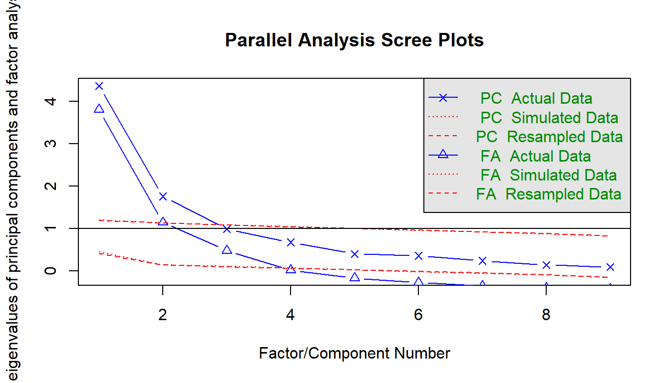
A scree plot is a line plot of the eigenvalues. An eigenvalue is the proportion of variance explained by each factor. Only factors with eigenvalues greater than those from uncorrelated data are useful. You want to find a sharp reduction in the size of the eigenvalues (like a cliff), with the rest of the smaller eigenvalues constituting rubble (scree!). After the eigenvalues drop dramatically in size, additional factors add relatively little to the information already extracted.
Parallel analysis helps to make the interpretation of scree plots more objective. The eigenvalues are plotted along with eigenvalues of simulated variables with population correlations of 0. The number of eigenvalues above the point where the two lines intersect is the suggested number of factors. The rationale for parallel analysis is that useful factors account for more variance than could be expected by chance.
psych::fa.parallel() compares a scree of your data set to a random data set to identify the number of factors. The elbow below here is at 3 factors.
Parallel analysis suggests that the number of factors = 3 and the number of components = 2
2.3.2 Exporatory Factor Analysis
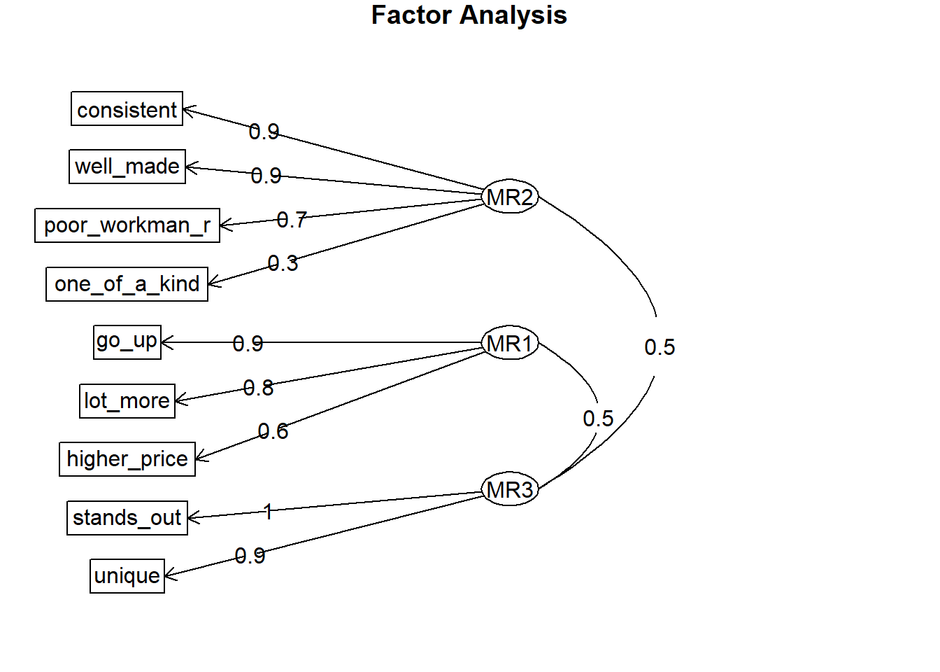
Use psych::fa() to perform the factor analysis with your chosen number of factors. The number of factors may be the result of your parallel analysis, or the opinion of the SMEs. In this case, we’ll go with the 3 factors identified by the parallel analysis.
Using EFA, you may tweak the number of factors or drop poorly-loading items. Each item should load highly to one and only one dimension. This one dimension is the item’s primary loading. Generally, a primary loading > .7 is excellent, >.6 is very good, >.5 is good, >.4 is fair, and <.4 is poor. Here are the factor loadings from the 3 factor model.
The brand-rep survey items load to 3 factors well except for the one_of_a_kind item. Its primary factor loading (0.309) is poor. The others are either very good (.6-.7) and excellent (>.7) range.
Look at the model eigenvalues. There should be one eigenvalue per dimension. Eigenvalues a little less than one may be contaminating the model.
Look at the factor score correlations. They should all be around 0.6. Much smaller means they are not describing the same latent variable. Much larger means they are describing the same dimension of the latent variable.
If you have a poorly loaded dimension, drop factors one at a time from the scale. one_of_a_kind loads across all three factors, but does not load strongly onto any one factor. one_of_a_kind is not clearly measuring any dimension of the latent variable. Drop it and try again.
The two-factor loading worked okay. The 4 factor loading only loaded one variable to the fourth factor. In this example the SME expected a three-factor model and the data did not contradict the theory, so stick with three.
Whereas the item generation phase tested for item equivalence, the EFA phase tests for internal reliability (consistency) of items. Internal reliability means the survey produces consistent results. The more common statistics for assessing internal reliability are Cronbach’s Alpha, and split-half.
2.3.3 Cronbach’s Alpha
In general, an alpha <.6 is unacceptable, <.65 is undesirable, <.7 is minimally acceptable, <.8 is respectable, <.9 is very good, and >=.9 suggests items are too alike. A very low alpha means items may not be measuring the same construct, so you should drop items. A very high alpha means items are multicollinear, and you should drop items. Here is Cronbach’s alpha for the brand reputation survey, after removing the poorly-loading one_of_a_kind variable.
psych::alpha(brand_rep[, 1:8])$total$std.alpha
[1] 0.8557356
This value is in the “very good” range. Cronbach’s alpha is often used to measure the reliability of a single dimension. Here are the values for the 3 dimensions.
Alpha is >0.7 for each dimension. Sometimes the alpha for our survey as a whole is greater than that of the dimensions. This can happen because Cronbach’s alpha is sensitive to the number of items. Over-inflation of the alpha statistic can be a concern when working with surveys containing a large number of items.
2.3.4 Split-Half
Use psych::splitHalf() to split the survey in half and test whether all parts of the survey contribute equally to measurement. This method is much less popular than Cronbach’s alpha.
psych::splitHalf(brand_rep[, 1:8])
Split half reliabilities
Call: psych::splitHalf(r = brand_rep[, 1:8])

Maximum split half reliability (lambda 4) =  0.93
Guttman lambda 6                          =  0.92
Average split half reliability            =  0.86
Guttman lambda 3 (alpha)                  =  0.86
Guttman lambda 2                          =  0.87
Minimum split half reliability  (beta)    =  0.66
Average interitem r =  0.43  with median =  0.4
2.4 Confirmatory Factor Analysis
Whereas EFA is used to develop a theory of the number of factors needed to explain the relationships among the survey items, confirmatory factor analysis (CFA) is a formal hypothesis test of the EFA theory. CFA measures construct validity, that is, whether you are really measuring what you claim to measure.
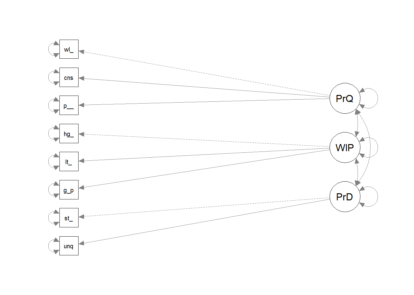
Use the lavaan package (latent variable analysis package), passing in the model definition. Here is the model for the three dimensions in the brand reputation survey. Lavaan’s default estimator is maximum likelihood, which assumes normality. You can change it to MLR which uses robust standard errors to mitigate non-normality. The summary prints a ton of output. Concentrate on the lambda - the factor loadings.
The CFA hypothesis test is a chi-square test, so is sensitive to normality assumptions and n-size. Other fit measure are reported too: * Comparative Fit Index (CFI) (look for value >.9) * Tucker-Lewis Index (TLI) (look for value >.9) * Root mean squared Error of Approximation (RMSEA) (look for value <.05)
There are actually 78 fit measures to choose from! Focus on CFI and TLI.
This output indicates a good model because both measures are >.9. Check the standardized estimates for each item. The standardized factor loadings are the basis of establishing construct validity. While we call these measures ‘loadings,’ they are better described as correlations of each manifest item with the dimensions. As you calculated, the difference between a perfect correlation and the observed is considered ‘error.’ This relationship between the so-called ‘true’ and ‘observed’ scores is the basis of classical test theory.
If you have a survey that meets your assumptions, performs well under EFA, but fails under CFA, return to your survey and revisit your scale, examine the CFA modification indices, factor variances, etc.
2.5 Convergent/Discriminant Validity
Construct validity means the survey measures what it intends to measure. It is composed of convergent validity and discriminant validity. Convergent validity means factors address the same concept. Discriminant validity means factors address different aspects of the concept.
Test for construct validity after assessing CFA model strength (with CFI, TFI, and RMSEA) – a poor-fitting model may have greater construct validity than a better-fitting model. Use the semTools::reliability() function. The average variance extracted (AVE) measures convergent validity (avevar) and should be > .5. The composite reliability (CR) measures discriminant validity (omega) and should be > .7.
These values look good for all three dimensions. As an aside, alpha is Cronbach’s alpha. Do not be tempted to test reliability and validity in the same step. Start with reliability because it is a necessary but insufficient condition for validity. By checking for internal consistency first, as measured by alpha, then construct validity, as measured by AVE and CR, you establish the necessary reliability of the scale as a whole was met, then took it to the next level by checking for construct validity among the unique dimensions.
At this point you have established that the latent and manifest variables are related as hypothesized, and that the survey measures what you intended to measure, in this case, brand reputation.
2.6 Replication
The replication phase establishes criterion validity and stability (reliability). Criterion validity is a measure of the relationship between the construct and some external measure of interest. Measure criterion validity with concurrent validity, how well items correlate with an external metric measured at the same time, and with predictive validity, how well an item predicts an external metric. Stability means the survey produces similar results over repeated test-retest administrations.
2.6.1 Criterion Validity
2.6.1.1 Concurrent Validity
Concurrent validity is a measure of whether our latent construct is significantly correlated to some outcome measured at the same time.
Suppose you have an additional data set of consumer spending on the brand. The consumer’s perception of the brand should correlate with their spending. Before checking for concurrent validity, standardize the data so that likert and other variable types are on the same scale.
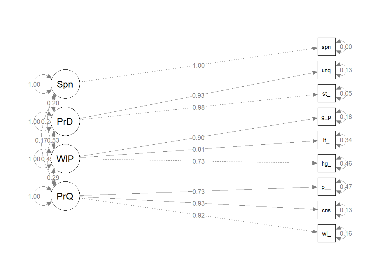
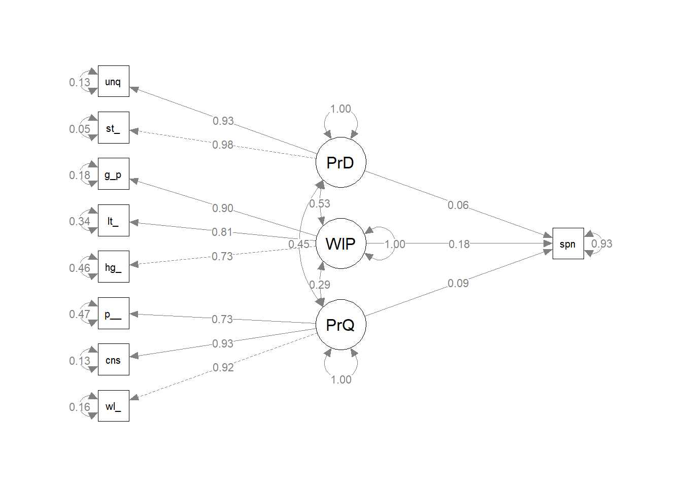
Do respondents with higher scores on our the brand reputation scale also tend to spend more at the store? Build model, and latentize spend as Spndng and model with the ~~ operator. Fit the model with the semTools::sem() function.
Here are the standardized covariances. Because the data is standardized, interpret these as correlations. The p-vales are not significant because the spending data was random.
Each dimension of brand reputation is positively correlated to spending history and the relationships are all significant.
2.6.1.2 Predictive Validity
Predictive validity is established by regressing some future outcome on your established construct. Assess predictive validity just as you would with any linear regression – regression estimates and p-values (starndardizedSolution()), and the r-squared coefficient of determination inspect().
Build a regression model with the single ~ operator. Then fit the model to the data as before.
There is a statistically significant relationship between one dimension of brand quality (Willingness to Pay) and spending. At this point you may want to drop the other two dimensions. However, the R^2 is not good - only 7% of the variability in Spending can be explained by the three dimension of our construct.
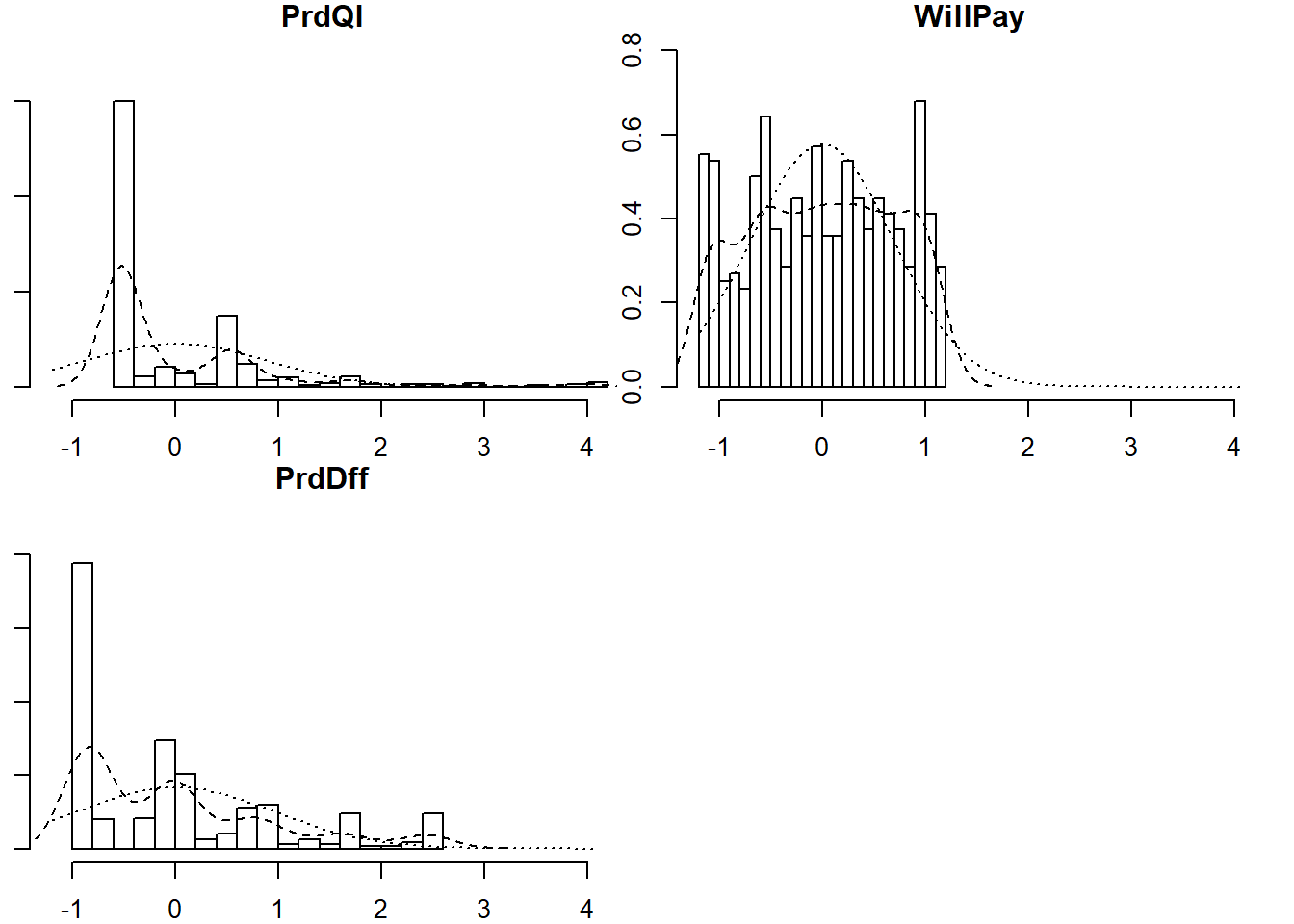
Factor scores represent individual respondents’ standing on a latent factor. While not used for scale validation per se, factor scores can be used for customer segmentation via clustering, network analysis and other statistical techniques.
brand_rep_cfa <- lavaan::cfa(brand_rep_pv_mdl, data = brand_rep_scaled)brand_rep_cfa_scores <- lavaan::predict(brand_rep_cfa) %>%as.data.frame()psych::describe(brand_rep_cfa_scores)
        vars   n mean   sd median trimmed  mad   min  max range  skew kurtosis
PrdQl      1 559    0 0.88  -0.50   -0.19 0.09 -0.57 4.02  4.59  2.31     6.18
WillPay    2 559    0 0.69   0.00    0.01 0.86 -1.15 1.16  2.31 -0.05    -1.18
PrdDff     3 559    0 0.96  -0.04   -0.15 1.17 -0.88 2.54  3.41  1.09     0.35
          se
PrdQl   0.04
WillPay 0.03
PrdDff  0.04
psych::multi.hist(brand_rep_cfa_scores)
map(brand_rep_cfa_scores, shapiro.test)
$PrdQl

    Shapiro-Wilk normality test

data:  .x[[i]]
W = 0.66986, p-value < 2.2e-16


$WillPay

    Shapiro-Wilk normality test

data:  .x[[i]]
W = 0.94986, p-value = 7.811e-13


$PrdDff

    Shapiro-Wilk normality test

data:  .x[[i]]
W = 0.82818, p-value < 2.2e-16
These scores are not normally distributed, which makes clustering a great choice for modeling factor scores. Clustering does not mean distance-based clustering, such as K-means, in this context. Mixture models consider data as coming from a distribution which itself is a mixture of clusters. To learn more about model-based clustering in the Hierarchical and Mixed Effects Models DataCamp course.
Factor scores can be extracted from a structural equation model and used as inputs in other models. For example, you can use the factor scores from the brand reputation dimensions as regressors for a regrssion on spending.
The coefficients and r-squared of the lm() and sem() models closely resemble each other, but keeping the regression inside the lavaan framework provides more information (as witnessed in the higher estimates and r-squared). A construct, once validated, can be combined with a wide range of outcomes and models to produce valuable information about consumer behavior and habits.
2.6.2 Test-Retest Reliability
Test-retest reliability is the ability to achieve the same result from a respondent at two closely-spaced points in time (repeated measures).
Suppose you had two surveys, identified by an id field.
If the correlation of scaled scores across time 1 and time 2 is greater than .9, that indicates very strong test-retest reliability. This measure can be difficult to collect because it requires the same respondents to answer the survey at two points in time. However, it’s a good technique to have in your survey development toolkit.
When validating a scale, it’s a good idea to split the survey results into two samples, using one for EFA and one for CFA. This works as a sort of cross-validation such that the overall fit of the model is less likely due to chance of any one sample’s makeup.
This section is aided by Fiona Middleton’s “Reliability vs. Validity in Research | Difference, Types and Examples” (Middleton 2022).↩︎
This section is primarily from George Mount’s Data Camp course (Mount, n.d.).↩︎
Source Code
# Item Selection {#sec-item-selection}```{r warning=FALSE, message=FALSE, include=FALSE}library(tidyverse)library(scales)```The design and analysis of a survey depends on its purpose. **Exploratory** surveys investigate topics with no particular expectation. They are usually qualitative and often ask open-ended questions which are analyzed for content (word/phrase frequency counts) and themes. **Descriptive** surveys measure the association between the survey topic(s) and the respondent attributes. They typically ask Likert scale questions. **Explanatory** surveys explain and quantify hypothesized relationships with inferential statistics.In a survey project, exploratory factor analysis (EFA), item reduction, and confirmatory factor analysis (CFA) play critical roles in refining and validating the questionnaire. Here’s how they fit into the major phases of a survey project:### 1. **Survey Design and Item Development** - **Item Generation**: During the initial design phase, you generate items (questions) based on the concepts you wish to measure. This involves creating questions that capture each domain or construct of interest. - **Preliminary Item Pool**: You often start with a larger pool of items than you plan to use in the final survey. The aim is to cover all relevant aspects of the constructs comprehensively, knowing that some items will be refined or removed later.### 2. **Pilot Testing and Exploratory Factor Analysis (EFA)** - **Pilot Survey Administration**: After developing the preliminary item pool, a pilot survey is administered to a small group from the target population. - **Exploratory Factor Analysis (EFA)**: EFA is conducted to explore the underlying structure of the data without imposing any predefined structure. This helps identify latent factors (or constructs) that the items represent and assess if the items group together as expected. - **Purpose**: EFA provides insights into whether items align with the hypothesized constructs or if adjustments are needed. - **Outcome**: The result of EFA often leads to item reduction, where redundant or low-loading items (items that don’t contribute well to the factors) are removed to create a cleaner, more interpretable structure.### 3. **Item Reduction and Refinement** - **Item Reduction**: Based on the results from EFA, items that don’t load well on any factor or that cause cross-loading issues (loading on multiple factors) are removed. This results in a streamlined set of items that reliably measure the intended constructs. - **Revised Survey Development**: A revised version of the survey is developed with the refined item pool, improving clarity, reducing redundancy, and ensuring that each item is relevant to a single construct.### 4. **Field Testing and Confirmatory Factor Analysis (CFA)** - **Larger Sample Administration**: The refined survey is then administered to a larger, more representative sample to test its reliability and validity. - **Confirmatory Factor Analysis (CFA)**: CFA is conducted to validate the factor structure identified in the EFA phase. CFA requires specifying the number of factors and their relationships based on prior knowledge or the EFA results. - **Purpose**: CFA tests how well the items fit the hypothesized structure and whether the constructs align with theoretical expectations. Good model fit in CFA indicates that the items reliably measure each intended factor.### 5. **Final Survey Administration and Data Collection** - With a validated survey, you can proceed to full-scale data collection, confident that the items are reliable and valid measures of the constructs.### 6. **Data Analysis and Reporting** - Following data collection, analysis is performed, often including descriptive statistics, correlations, and further structural equation modeling if needed. - **Reporting**: The results and insights gained through EFA, item reduction, and CFA help demonstrate the survey's validity and reliability, which is crucial when presenting findings to stakeholders.Each of these steps is important to ensure that the survey effectively measures the constructs of interest, minimizes measurement error, and provides meaningful insights for your study or project.## Reliability and ValidityA high quality survey will be both reliable (consistent) and valid (accurate).[^01-item_selection-1] A reliable survey is reproducible under similar conditions. It produces consistent results across time, samples, and sub-samples within the survey itself. Reliable surveys are not necessarily *accurate* though. A valid survey accurately measures its latent variable. Its results are compatible with established theory and with other measures of the concept. Valid surveys are usually reliable too.[^01-item_selection-1]: This section is aided by Fiona Middleton's "Reliability vs. Validity in Research \| Difference, Types and Examples" [@middleton2022].**Reliability** can entail one or more of the following:- **Inter-rater reliability (aka Equivalence)**. Each survey item is unambiguous, so subject matter experts should respond identically. This applies to opinion surveys of factual concepts, not personal preference surveys. E.g., two psychologists completing a survey assessing a patient's mental health should respond identically. Use the Cohen's Kappa test of inter-rater reliability to test equivalence (*see* Section \@ref(itemgeneration) on item generation).- **Internal consistency**. Survey items measuring the same latent variable are highly correlated. Use the Cronbach alpha test and split-half test to assess internal consistency (*see* Section \@ref(itemreduction) on item reduction).- **Stability (aka Test-retest)**. Repeated measurements yield the same results. You use the test-retest construct to assess stability in the *Replication* phase.There are three assessments of **validity**:- **Content validity**. The survey items cover *all* aspects of the latent variable. Use Lawshe's CVR to assess content validity (*see* Section \@ref(itemgeneration) on item generation).- **Construct validity**. The survey items are properly grounded on a theory of the latent variable. Use convergent analysis and discriminant analysis to assess construct validity in the *Convergent/Discriminant Validity* phase.- **Criterion validity**. The survey item results correspond to other valid measures of the same latent variable. Use concurrent analysis and predictive analysis to assess criterion validity in the *Replication* phase.Survey considerations- Question order, selection order- respondent burden and fatigueQuality of Measurement: Reliability and Validity (internal and external)Pretest and pilot testProbability Sampling: - simple random, systematic random, stratified random, cluster, and multistate cluster. - power analysisReporting - Descriptive statistics - Write-upContinuous latent variables (e.g., level of satisfaction) can be measured with factor analysis (exploratory and confirmatory) or item response theory (IRT) models. Categorical or discrete variables (e.g., market segment) can be modeled with latent class analysis (LCA) or latent mixture modeling. You can even combine models, e.g., satisfaction within market segment.In practice, you specify the model, evaluate the fit, then revise the model or add/drop items from the survey.A full survey project usually consists of six phases.[^01-item_selection-2][^01-item_selection-2]: This section is primarily from George Mount's Data Camp course [@mount].1. **Item Generation** (Section \@ref(itemgeneration)). Start by generating a list of candidate survey items. With help from SMEs, you evaluate the equivalence (interrater reliability) and content validity of the candidate survey items and pare down the list into the final survey.2. **Survey Administration** (Section \@ref(surveyadministration)). Administer the survey to respondents and perform an exploratory data analysis. Summarize the Likert items with plots and look for correlations among the variables.3. **Item Reduction** (Section \@ref(itemreduction)). Explore the dimensions of the latent variable in the survey data with parallel analysis and exploratory factor analysis. Assess the internal consistency of the items with Cronbach's alpha and split-half tests, and remove items that do not add value and/or amend your theory of the number of dimensions.4. **Confirmatory Factor Analysis** (Section \@ref(confirmatoryfactoranalysis)). Perform a formal hypothesis test of the theory that emerged from the exploratory factor analysis.5. **Convergent/Discriminant Validity** (Section \@ref(convergentvalidity)). Test for convergent and discriminant construct validity.6. **Replication** (Section \@ref(replication)). Establish test-retest reliability and criterion validity.## Item Generation {#itemgeneration}Define your latent variable(s), that is, the unquantifiable variables you intend to infer from variables you *can* quntify. E.g., "Importance of 401(k) matching"After you generate a list of candidate survey items, enlist SMEs to assess their inter-rater reliability with *Cohen's Kappa* and content validity with *Lawshe's CVR*.### Cohen's KappaAn item has inter-rater reliability if it produces consistent results across raters. One way to test this is by having SMEs take the survey. Their answers should be close to each other. Conduct an inter-rater reliability test by measuring the statistical significance of SME response agreement using the Kohen's kappa test statistic.Suppose your survey measures brand loyalty and two SMEs answer 13 survey items like this. The SMEs agreed on 6 of the 13 items (46%).```{r include=FALSE}sme <- data.frame( RATER_A = c(1, 2, 3, 2, 1, 1, 1, 2, 3, 3, 2, 1, 1), RATER_B = c(1, 2, 2, 3, 3, 1, 1, 1, 2, 3, 3, 3, 1))sme2 <- sme %>% mutate(RATER_B = if_else(RATER_A == 1 & RATER_B == 3, 2, RATER_B))``````{r paged.print=TRUE}sme %>% mutate(agreement = RATER_A == RATER_B)```You could measure SME agreement with a simple correlation matrix (`cor(sme)`) or by measuring the percentage of items they rate identically (`irr::agree(sme)`), but these measures do not test for statistical validity.```{r collapse=TRUE}cor(sme)irr::agree(sme)```Instead, calculate the Kohen's kappa test statistic, $\kappa$, to assess statistical validity. Cohen's kappa compares the observed agreement (accuracy) to the probability of chance agreement. $\kappa$ \>= 0.8 is very strong agreement, $\kappa$ \>= 0.6 substantial, $\kappa$ \>= 0.4 moderate, and $\kappa$ \< 0.4 is poor agreement. In this example, $\kappa$ is only 0.32 (poor agreement).```{r}psych::cohen.kappa(sme)psych::cohen.kappa(sme2)```Use the weighted kappa for ordinal measures like Likert items (*see* [Wikipedia](https://en.wikipedia.org/wiki/Cohen%27s_kappa)).### Lawshe's CVRAn item has content validity if SMEs agree on its relevance to the latent variable. Test content validity with Lawshe's content validity ratio (CVR),$$CVR = \frac{E - N/2}{N/2}$$ where $N$ is the number of SMEs and $E$ is the number who rate the item as *essential*. CVR can range from -1 to 1. E.g., suppose three SMEs (A, B, and C) assess the relevance of 5 survey items as "Not Necessary", "Useful", or "Essential":```{r echo=FALSE}sme2 <- data.frame( item = c(1:5), A = c("Essential", "Useful", "Not necesary", "Essential", "Essential"), B = c("Useful", "Not necesary", "Not necesary", "Useful", "Essential"), C = c("Not necesary", "Useful", "Essential", "Essential", "Essential"))print(sme2)```Use the `psychometric::CVratio()` function to calculate CVR. The threshold *CVR* to keep or drop an item depends on the number of raters. CVR should be \>= 0.99 for 5 experts; \>= 0.49 for 15, and \>= 0.29 for 40.```{r}sme2 %>%pivot_longer(-item, names_to ="expert", values_to ="rating") %>%group_by(item) %>%summarize(.groups ="drop",n_sme =length(unique(expert)),n_ess =sum(rating =="Essential"),CVR = psychometric::CVratio(NTOTAL = n_sme, NESSENTIAL = n_ess))```In this example, items vary widely in content validity from unanimous consensus for to unanimous consensus against.## Item Reduction {#itemreduction}The third phase, explores the mapping of the factors (aka "manifest variables") to the latent variable's "dimensions" and refines the survey to exclude factors that do not map to a dimension. A latent variable may have several dimensions. E.g., "brand loyalty" may consist of "brand identification", "perceived value", and "brand trust". Exploratory factor analysis (EFA), identifies the dimensions in the data, and whether any items do *not* reveal information about the latent variable. EFA establishes the *internal reliability*, whether similar items produce similar scores.Start with a parallel analysis and scree plot. This will suggest the number of factors in the data. Use this number as the input to an exploratory factor analysis.### Parallel AnalysisA [scree plot](https://www.sciencedirect.com/topics/mathematics/scree-plot) is a line plot of the eigenvalues. An eigenvalue is the proportion of variance explained by each factor. Only factors with eigenvalues greater than those from uncorrelated data are useful. You want to find a sharp reduction in the size of the eigenvalues (like a cliff), with the rest of the smaller eigenvalues constituting rubble (scree!). After the eigenvalues drop dramatically in size, additional factors add relatively little to the information already extracted.Parallel analysis helps to make the interpretation of scree plots more objective. The eigenvalues are plotted along with eigenvalues of simulated variables with population correlations of 0. The number of eigenvalues above the point where the two lines intersect is the suggested number of factors. The rationale for parallel analysis is that useful factors account for more variance than could be expected by chance.`psych::fa.parallel()` compares a scree of your data set to a random data set to identify the number of factors. The elbow below here is at 3 factors.```{r fig.height=4}brand_rep <- read_csv(url("https://assets.datacamp.com/production/repositories/4494/datasets/59b5f2d717ddd647415d8c88aa40af6f89ed24df/brandrep-cleansurvey-extraitem.csv"))psych::fa.parallel(brand_rep)```### Exporatory Factor AnalysisUse `psych::fa()` to perform the factor analysis with your chosen number of factors. The number of factors may be the result of your parallel analysis, or the opinion of the SMEs. In this case, we'll go with the 3 factors identified by the parallel analysis.```{r}brand_rep_efa <- psych::fa(brand_rep, nfactors =3)# psych::scree(brand_rep) # psych makes scree plot's too.psych::fa.diagram(brand_rep_efa)```Using EFA, you may tweak the number of factors or drop poorly-loading items. Each item should load highly to one and only one dimension. This one dimension is the item's primary loading. Generally, a primary loading \> .7 is excellent, \>.6 is very good, \>.5 is good, \>.4 is fair, and \<.4 is poor. Here are the factor loadings from the 3 factor model.```{r}brand_rep_efa$loadings```The brand-rep survey items load to 3 factors well except for the `one_of_a_kind` item. Its primary factor loading (0.309) is poor. The others are either very good (.6-.7) and excellent (\>.7) range.Look at the model eigenvalues. There should be one eigenvalue per dimension. Eigenvalues a little less than one may be contaminating the model.```{r}brand_rep_efa$e.value```Look at the factor score correlations. They should all be around 0.6. Much smaller means they are not describing the same latent variable. Much larger means they are describing the same dimension of the latent variable.```{r}brand_rep_efa$r.scores```If you have a poorly loaded dimension, drop factors one at a time from the scale. `one_of_a_kind` loads across all three factors, but does not load strongly onto any one factor. `one_of_a_kind` is not clearly measuring any dimension of the latent variable. Drop it and try again.```{r}brand_rep_efa <- psych::fa(brand_rep %>%select(-one_of_a_kind), nfactors =3)brand_rep_efa$loadingsbrand_rep_efa$e.valuebrand_rep_efa$r.scores```This is better. We have three dimensions of brand reputation:- items `well_made`, `consistent`, and `poor_workman_r` describe *Product Quality*,- items `higher_price`, `lot_more`, and `go_up` describe *Willingness to Pay*, and- items `stands_out` and `unique` describe *Product Differentiation*Even if the data and your theory suggest otherwise, explore what happens when you include more or fewer factors in your EFA.```{r}psych::fa(brand_rep, nfactors =2)$loadingspsych::fa(brand_rep, nfactors =4)$loadings```The two-factor loading worked okay. The 4 factor loading only loaded one variable to the fourth factor. In this example the SME expected a three-factor model and the data did not contradict the theory, so stick with three.Whereas the item generation phase tested for item equivalence, the EFA phase tests for internal reliability (*consistency*) of items. Internal reliability means the survey produces consistent results. The more common statistics for assessing internal reliability are Cronbach's Alpha, and split-half.### Cronbach's AlphaIn general, an alpha \<.6 is unacceptable, \<.65 is undesirable, \<.7 is minimally acceptable, \<.8 is respectable, \<.9 is very good, and \>=.9 suggests items are *too* alike. A very low alpha means items may not be measuring the same construct, so you should drop items. A very high alpha means items are multicollinear, and you should drop items. Here is Cronbach's alpha for the brand reputation survey, after removing the poorly-loading `one_of_a_kind` variable.```{r}psych::alpha(brand_rep[, 1:8])$total$std.alpha```This value is in the "very good" range. Cronbach's alpha is often used to measure the reliability of a single dimension. Here are the values for the 3 dimensions.```{r collapse=TRUE}psych::alpha(brand_rep[, 1:3])$total$std # Product Qualitypsych::alpha(brand_rep[, 4:6])$total$std # Willingness to Paypsych::alpha(brand_rep[, 7:8])$total$std # Product Differentiation```Alpha is \>0.7 for each dimension. Sometimes the alpha for our survey as a whole is greater than that of the dimensions. This can happen because Cronbach's alpha is sensitive to the number of items. Over-inflation of the alpha statistic can be a concern when working with surveys containing a large number of items.### Split-HalfUse `psych::splitHalf()` to split the survey in half and test whether all parts of the survey contribute equally to measurement. *This method is much less popular than Cronbach's alpha.*```{r}psych::splitHalf(brand_rep[, 1:8])```## Confirmatory Factor Analysis {#confirmatoryfactoranalysis}Whereas EFA is used to develop a theory of the number of factors needed to explain the relationships among the survey items, confirmatory factor analysis (CFA) is a formal hypothesis test of the EFA theory. CFA measures construct validity, that is, whether you are really measuring what you claim to measure.These notes explain how to use CFA, but do not explain the theory. For that you need to learn about [dimensionality reduction](https://www.datacamp.com/courses/dimensionality-reduction-in-r), and [structural equation modeling](https://www.datacamp.com/courses/structural-equation-modeling-with-lavaan-in-r).Use the **lavaan** package (latent variable analysis package), passing in the model definition. Here is the model for the three dimensions in the brand reputation survey. Lavaan's default estimator is maximum likelihood, which assumes normality. You can change it to MLR which uses robust standard errors to mitigate non-normality. The summary prints a ton of output. Concentrate on the `lambda` - the factor loadings.```{r}brand_rep_mdl <-paste("PrdQl =~ well_made + consistent + poor_workman_r","WillPay =~ higher_price + lot_more + go_up","PrdDff =~ stands_out + unique", sep ="\n")brand_rep_cfa <- lavaan::cfa(model = brand_rep_mdl, data = brand_rep[, 1:8], estimator ="MLR")# lavaan::summary(brand_rep_cfa, fit.measures = TRUE, standardized = TRUE)semPlot::semPaths(brand_rep_cfa, rotation =4)lavaan::inspect(brand_rep_cfa, "std")$lambda```The CFA hypothesis test is a chi-square test, so is sensitive to normality assumptions and n-size. Other fit measure are reported too: \* Comparative Fit Index (CFI) (look for value \>.9) \* Tucker-Lewis Index (TLI) (look for value \>.9) \* Root mean squared Error of Approximation (RMSEA) (look for value \<.05)There are actually `r length(lavaan::fitMeasures(brand_rep_cfa))` fit measures to choose from! Focus on CFI and TLI.```{r}lavaan::fitMeasures(brand_rep_cfa, fit.measures =c("cfi", "tli"))```This output indicates a good model because both measures are \>.9. Check the standardized estimates for each item. The standardized factor loadings are the basis of establishing construct validity. While we call these measures 'loadings,' they are better described as correlations of each manifest item with the dimensions. As you calculated, the difference between a perfect correlation and the observed is considered 'error.' This relationship between the so-called 'true' and 'observed' scores is the basis of classical test theory.```{r}lavaan::standardizedSolution(brand_rep_cfa) %>%filter(op =="=~") %>%select(lhs, rhs, est.std, pvalue)```If you have a survey that meets your assumptions, performs well under EFA, but fails under CFA, return to your survey and revisit your scale, examine the CFA modification indices, factor variances, etc.## Convergent/Discriminant Validity {#convergentvalidity}Construct validity means the survey measures what it intends to measure. It is composed of convergent validity and discriminant validity. Convergent validity means factors address the same concept. Discriminant validity means factors address different aspects of the concept.Test for construct validity *after* assessing CFA model strength (with CFI, TFI, and RMSEA) -- a poor-fitting model may have greater construct validity than a better-fitting model. Use the `semTools::reliability()` function. The average variance extracted (AVE) measures convergent validity (`avevar`) and should be \> .5. The composite reliability (CR) measures discriminant validity (`omega`) and should be \> .7.```{r}semTools::reliability(brand_rep_cfa)```These values look good for all three dimensions. As an aside, `alpha` is Cronbach's alpha. Do not be tempted to test reliability and validity in the same step. Start with reliability because it is a necessary but insufficient condition for validity. By checking for internal consistency first, as measured by alpha, then construct validity, as measured by AVE and CR, you establish the necessary reliability of the scale as a whole was met, then took it to the next level by checking for construct validity among the unique dimensions.At this point you have established that the latent and manifest variables are related as hypothesized, and that the survey measures what you intended to measure, in this case, brand reputation.## Replication {#replication}The replication phase establishes criterion validity and stability (reliability). Criterion validity is a measure of the relationship between the construct and some external measure of interest. Measure criterion validity with *concurrent validity*, how well items correlate with an external metric measured at the same time, and with *predictive validity*, how well an item predicts an external metric. Stability means the survey produces similar results over repeated *test-retest* administrations.### Criterion Validity#### Concurrent ValidityConcurrent validity is a measure of whether our latent construct is significantly correlated to some outcome measured at the same time.Suppose you have an additional data set of consumer spending on the brand. The consumer's perception of the brand should correlate with their spending. Before checking for concurrent validity, standardize the data so that likert and other variable types are on the same scale.```{r}set.seed(20201004)brand_rep <- brand_rep %>%mutate(spend = ((well_made + consistent + poor_workman_r)/3*5+ (higher_price + lot_more + go_up)/3*3+ (stands_out + unique)/2*2) /10)brand_rep$spend <- brand_rep$spend +rnorm(559, 5, 4) # add randomnessbrand_rep_scaled <-scale(brand_rep)```Do respondents with higher scores on our the brand reputation scale also tend to spend more at the store? Build model, and latentize `spend` as `Spndng` and model with the `~~` operator. Fit the model with the `semTools::sem()` function.```{r}brand_rep_cv_mdl <-paste("PrdQl =~ well_made + consistent + poor_workman_r","WillPay =~ higher_price + lot_more + go_up","PrdDff =~ stands_out + unique","Spndng =~ spend","Spndng ~~ PrdQl + WillPay + PrdDff",sep ="\n")brand_rep_cv <- lavaan::sem(data = brand_rep_scaled, model = brand_rep_cv_mdl)```Here are the standardized covariances. Because the data is standardized, interpret these as correlations. The p-vales are not significant because the spending data was random.```{r}lavaan::standardizedSolution(brand_rep_cv) %>%filter(rhs =="Spndng") %>%select(-op, -rhs)semPlot::semPaths(brand_rep_cv, whatLabels ="est.std", edge.label.cex = .8, rotation =2)```Each dimension of brand reputation is positively correlated to spending history and the relationships are all significant.#### Predictive ValidityPredictive validity is established by regressing some future outcome on your established construct. Assess predictive validity just as you would with any linear regression -- regression estimates and p-values (`starndardizedSolution()`), and the r-squared coefficient of determination `inspect()`.Build a regression model with the single `~` operator. Then fit the model to the data as before.```{r}brand_rep_pv_mdl <-paste("PrdQl =~ well_made + consistent + poor_workman_r","WillPay =~ higher_price + lot_more + go_up","PrdDff =~ stands_out + unique","spend ~ PrdQl + WillPay + PrdDff",sep ="\n")brand_rep_pv <- lavaan::sem(data = brand_rep_scaled, model = brand_rep_pv_mdl)#lavaan::summary(brand_rep_pv, standardized = T, fit.measures = T, rsquare = T)semPlot::semPaths(brand_rep_pv, whatLabels ="est.std", edge.label.cex = .8, rotation =2)lavaan::standardizedSolution(brand_rep_pv) %>%filter(op =="~") %>%mutate_if(is.numeric, round, digits =3)lavaan::inspect(brand_rep_pv, "r2")```There is a statistically significant relationship between one dimension of brand quality (Willingness to Pay) and spending. At this point you may want to drop the other two dimensions. However, the R\^2 is not good - only 7% of the variability in Spending can be explained by the three dimension of our construct.Factor scores represent individual respondents' standing on a latent factor. While not used for scale validation per se, factor scores can be used for customer segmentation via clustering, network analysis and other statistical techniques.```{r test385}brand_rep_cfa <- lavaan::cfa(brand_rep_pv_mdl, data = brand_rep_scaled)brand_rep_cfa_scores <- lavaan::predict(brand_rep_cfa) %>% as.data.frame()psych::describe(brand_rep_cfa_scores)psych::multi.hist(brand_rep_cfa_scores)map(brand_rep_cfa_scores, shapiro.test)```These scores are not normally distributed, which makes clustering a great choice for modeling factor scores. Clustering does not mean distance-based clustering, such as K-means, in this context. Mixture models consider data as coming from a distribution which itself is a mixture of clusters. To learn more about model-based clustering in the [Hierarchical and Mixed Effects Models](https://www.datacamp.com/courses/hierarchical-and-mixed-effects-models) DataCamp course.Factor scores can be extracted from a structural equation model and used as inputs in other models. For example, you can use the factor scores from the brand reputation dimensions as regressors for a regrssion on spending.```{r test397}brand_rep_fs_reg_dat <- bind_cols(brand_rep_cfa_scores, spend = brand_rep$spend)brand_rep_fs_reg <- lm(spend ~ PrdQl + WillPay + PrdDff, data = brand_rep_fs_reg_dat)summary(brand_rep_fs_reg)$coef```The coefficients and r-squared of the lm() and sem() models closely resemble each other, but keeping the regression inside the lavaan framework provides more information (as witnessed in the higher estimates and r-squared). A construct, once validated, can be combined with a wide range of outcomes and models to produce valuable information about consumer behavior and habits.### Test-Retest ReliabilityTest-retest reliability is the ability to achieve the same result from a respondent at two closely-spaced points in time (repeated measures).Suppose you had two surveys, identified by an `id` field.```{r test411}# svy_1 <- brand_rep[sample(1:559, 300),] %>% as.data.frame()# svy_2 <- brand_rep[sample(1:559, 300),] %>% as.data.frame()# survey_test_retest <- psych::testRetest(t1 = svy_1, t2 = svy_2, id = "id")# survey_test_retest$r12```An r\^2 \<.7 is unacceptable, \<.9 good, and \>.9 very good. This one is unacceptable.One way to check for replication is by splitting the data in half.```{r test422}# svy <- bind_rows(svy_1, svy_2, .id = "time")# # psych::describeBy(svy, "time")# # brand_rep_test_retest <- psych::testRetest(# t1 = filter(svy, time == 1),# t2 = filter(svy, time == 2),# id = "id")# # brand_rep_test_retest$r12```If the correlation of scaled scores across time 1 and time 2 is greater than .9, that indicates very strong test-retest reliability. This measure can be difficult to collect because it requires the same respondents to answer the survey at two points in time. However, it's a good technique to have in your survey development toolkit.When validating a scale, it's a good idea to split the survey results into two samples, using one for EFA and one for CFA. This works as a sort of cross-validation such that the overall fit of the model is less likely due to chance of any one sample's makeup.```{r}# brand_rep_efa_data <- brand_rep[1:280,]# brand_rep_cfa_data <- brand_rep[281:559,]# # efa <- psych::fa(brand_rep_efa_data, nfactors = 3)# efa$loadings# # brand_rep_cfa <- lavaan::cfa(brand_rep_mdl, data = brand_rep_cfa_data)# lavaan::inspect(brand_rep_cfa, what = "call")# # lavaan::fitmeasures(brand_rep_cfa)[c("cfi","tli","rmsea")]```