6  Statistical Testing

library(tidyverse)
library(scales)
library(janitor)
library(survey)
library(srvyr)
library(gtsummary)

6.1 T-Test

Use t-tests to compare two proportions or means. The difference between t-tests with non-survey data and survey data is based on the underlying variance estimation difference. survey::svyttest() handles sample weights.

Continuous

Test whether api00 differs from 600.

svyttest(
  formula = api00 - 600 ~ 0,
  design = apisrs_des,
  na.rm = TRUE
)

    Design-based one-sample t-test

data:  api00 - 600 ~ 0
t = 6.1175, df = 198, p-value = 4.992e-09
alternative hypothesis: true mean is not equal to 0
95 percent confidence interval:
 38.34439 74.82561
sample estimates:
  mean 
56.585 

Proportion

Test whether growth > 0 on average.

svyttest(
  formula = (growth > 0) ~ 0,
  design = apisrs_des,
  na.rm = TRUE
)

    Design-based one-sample t-test

data:  (growth > 0) ~ 0
t = 39.781, df = 198, p-value < 2.2e-16
alternative hypothesis: true mean is not equal to 0
95 percent confidence interval:
 0.841129 0.928871
sample estimates:
 mean 
0.885 

Test whether growth is higher for high school than for others.

svyttest(
  growth ~ (stype == "H"),
  design = apisrs_des
)

    Design-based t-test

data:  growth ~ (stype == "H")
t = -5.5339, df = 198, p-value = 9.845e-08
alternative hypothesis: true difference in mean is not equal to 0
95 percent confidence interval:
 -29.73118 -14.10882
sample estimates:
difference in mean 
            -21.92 

6.2 Chi-Squared Test

Goodness of Fit

Does meals_cut distribution match hypothesized population [.25, .25, .5]?

gof <- svygofchisq(
  formula = ~meals_cut,
  p = c(.25, .25, .5),
  design = apistrat_des,
  na.rm = TRUE
)

gof

    Design-based chi-squared test for given probabilities

data:  ~meals_cut
X-squared = 1100.4, scale = 31.6017, df = 1.6449, p-value = 1.438e-08

apistrat_des |> 
  summarize(
    .by = hsg_cut,
    observed = survey_mean(vartype = "ci")
  ) |>
  mutate(expected = c(.25, .25, .5)) |>
  pivot_longer(c(observed, expected), values_to = "Proportion") |>
  ggplot(aes(x = hsg_cut)) +
  geom_errorbar(aes(ymin = observed_low, ymax = observed_upp), width = .5) +
  geom_point(aes(y = Proportion, color = name), size = 2) +
  theme(legend.position = "top", legend.justification = "left") +
  labs(color = NULL)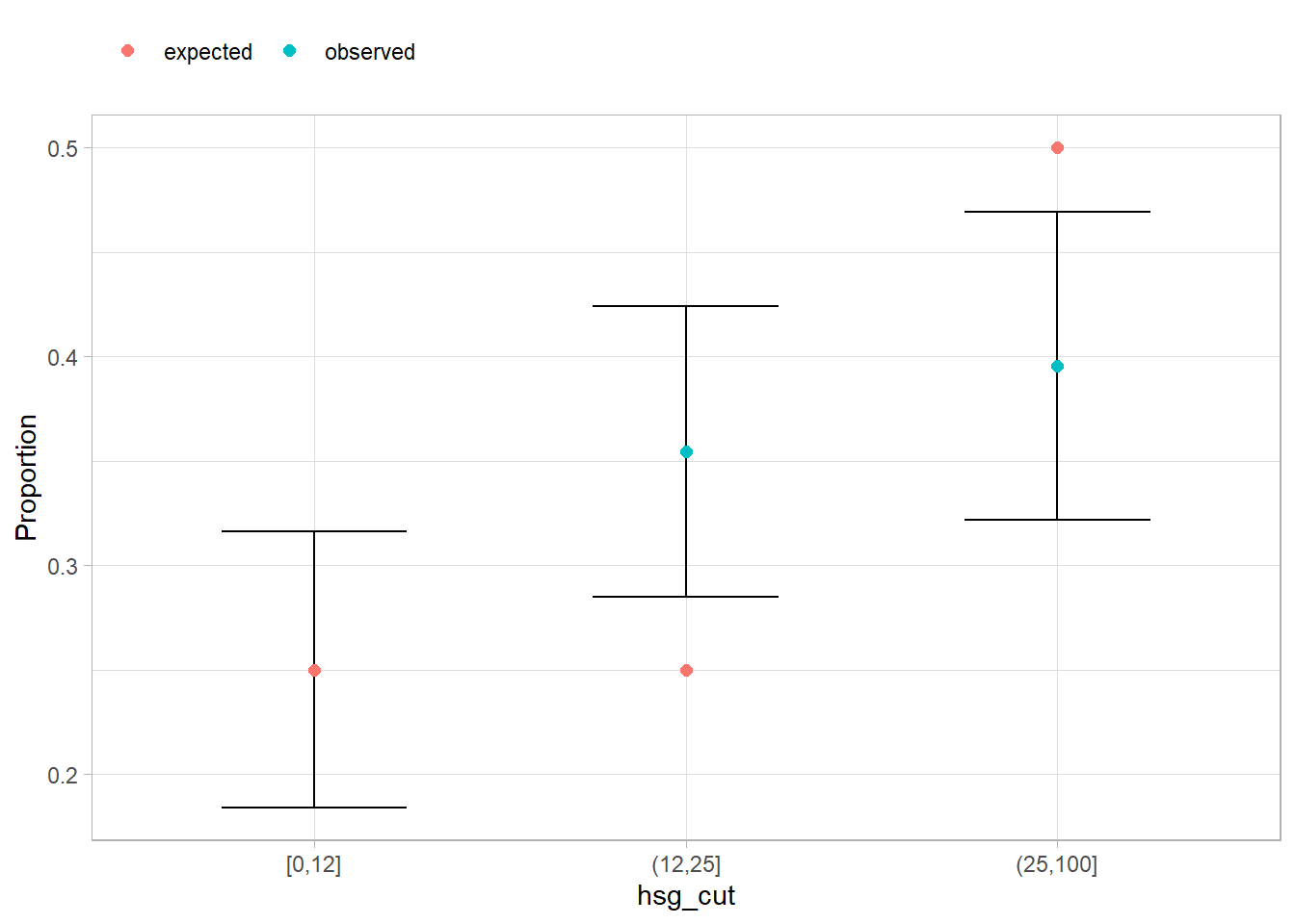

Test of Independence

Is meals_cut distribution related to hsg_cut?

svychisq(
  formula = ~ meals_cut + hsg_cut,
  design = apistrat_des,
  statistic = "Wald",
  na.rm = TRUE
)

    Design-based Wald test of association

data:  NextMethod()
F = 9.4761, ndf = 4, ddf = 197, p-value = 5.01e-07

gtsummary does not have a cross table function, but you can make your own.

apistrat_des |>
  drop_na(meals_cut, hsg_cut) |>
  group_by(meals_cut, hsg_cut) |>
  summarize(Obs = round(survey_mean(vartype = "ci"), 3), .groups = "drop") |>
  mutate(prop = glue::glue("{Obs} ({Obs_low}, {Obs_upp})")) |>
  pivot_wider(id_cols = meals_cut, names_from = hsg_cut, values_from = prop) |>
  gt::gt(rowname_col = "Meals") |>
  gt::tab_stubhead("High School Grad")

meals_cut	[0,12]	(12,25]	(25,100]
[0,12]	0.797 (0.642, 0.952)	0.129 (0.007, 0.252)	0.073 (-0.035, 0.182)
(12,25]	0.35 (0.175, 0.526)	0.453 (0.278, 0.628)	0.197 (0.06, 0.333)
(25,100]	0.127 (0.064, 0.189)	0.374 (0.288, 0.46)	0.499 (0.409, 0.59)

Test of Homogeneity

Is the distribution of meals_cut the same for each level of hsg_cut?

svychisq(
  formula = ~ meals_cut + hsg_cut,
  design = apistrat_des,
  statistic = "Chisq",
  na.rm = TRUE
)

    Pearson's X^2: Rao & Scott adjustment

data:  NextMethod()
X-squared = 59.835, df = 4, p-value = 1.63e-11